Ron Kohavi is somewhat of a prominent figure in the A/B testing community. Armed with having coauthored “Trustworthy Online Controlled Experiments”, experience at places like AirBNB and Microsoft, and what seems to be a $20/month subscription to ChatGPT, he will often post these kinds of questions on LinkedIn.
The post below really caught my attention (probably because of the AI generated accompanying picture, a fad everyone seems to be doing for some reason).
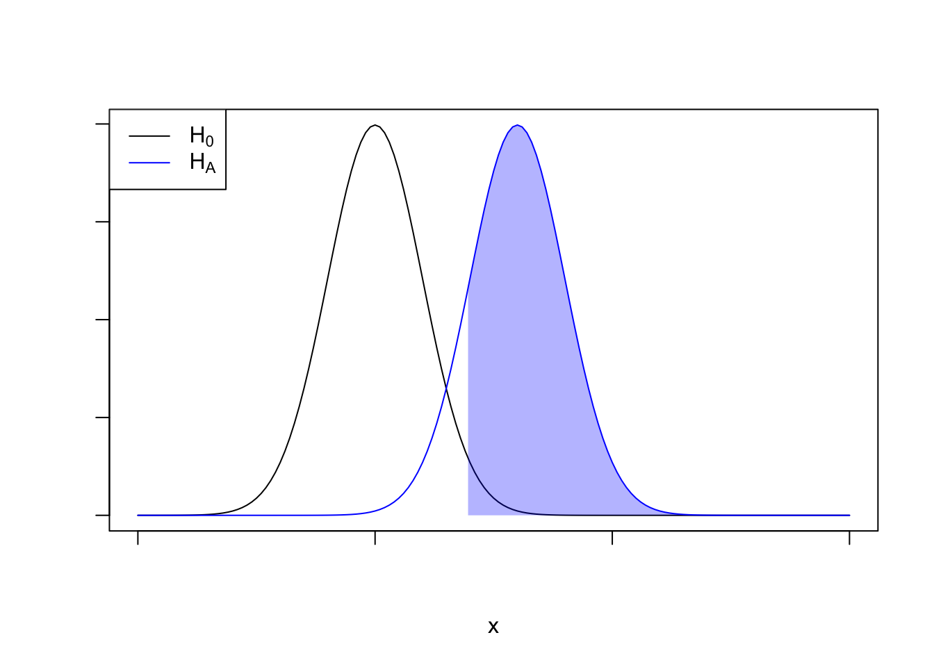
This should be fairly simple to reason through. Below is a plot depicting the concept of statistical power. The black curve is the sampling distribution under the null, the blue curve is the sampling distribution under the alternative implied by the minimal detectable effect (MDE). The area under the blue curve is the statsitical power (its the probability we observe a test statistic greater than the critical value).
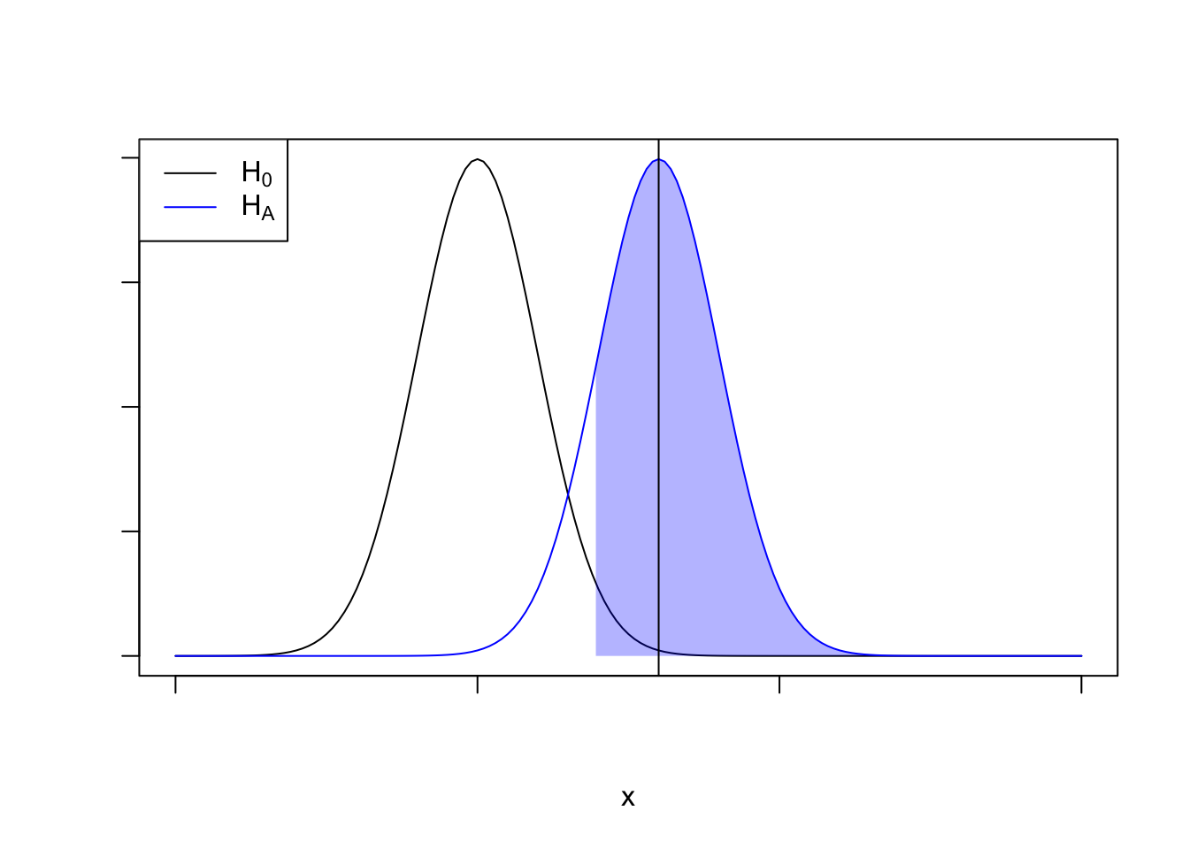
According to Ron, we run our experiment and observe the our (MDE) exactly. In our picture, that means we observe the mean of the sampling distribution under the alternative, so we just need to find how far out the MDE is with respect to the null distribution.
Let’s do a little bit of math. Assuming the sampling distribution under the null is standard normal, the critical value would be \(\mu_0 + \sigma_0z_{1-\alpha}\). The critical value under the alternative would then be \(\mu_1 + z_{1-\beta}\sigma_1\). Plugging in some numbers, this means the mean under the alternative should have a z-zcore of \(\mu_0 + \sigma_0z_{1-\alpha} - \sigma_1z_{1-\beta}\). Now, we just need to evaluate \(1 - \mathbf{\Phi}(\mu_0 + \sigma_0z_{1-\alpha} - \sigma_1z_{1-\beta})\).
Assume that these distributions are standardized so that \(\mu_0 = 0\) and \(\sigma_0 = \sigma_1=1\). This results in a p-value of
pnorm(2.8, lower.tail = F)
[1] 0.00255513
and I bet because I’ve only focused on one tail I should multiply by 2, so a p value of ~ 0.005, which seems to be correct.