Survival Analysis With Logistic Regression

This question came up on cross validated. In the course of responding to my answer, OP asks “why can’t I adjust for exposure length in a logistic regression” which kind of got me scratching my head. Seems like it could be done.

I brought the question to twitter, and Dr. Ellie Murray responded reminding me that time to death and death are different outcomes and should be treated differently. A logistic regression could be done, depending on what you’re trying to model.

Finally, Frank Harrell responded to Dr. Murray, with a link to a paper by Brad Efron (because of course Efron wrote something on this) which showed how this can be done quite elegantly.

Let’s see how we can use logistic regression for survival analysis.

The Gist

Recall that the Kaplan-Meir product limit estimator looks like

\[ \widehat{S}_{KM} (t) = \prod_{i: t_i \leq t} \left(1-\dfrac{d_i}{n_i} \right) \>. \]

Here, \(d_i\) is the number of subjects who experience the outcome at time \(t_i\), and \(n_i\) is the number of individuals known to have survived up to time \(t_i\). In essence, the product limit estimator is a product of a sequence of probabilities. What else do we use to model probabilities? Logistic regression.

Efron writes that the main assumption for using logistic regression to model these probabilities is that the number of events \(d_i\) is binomial given \(n_i\)

\[ d_i \mid n_i \sim \operatorname{Binomial}(h_i; n_i) \>. \]

Here, \(h_i\) is the discrete hazard rate (i.e. the probability the subject experiences the outcome during the \(i^{th}\) interval given the subject has survived until the beginning of the \(i^{th}\) interval).

The main problem is that the hazard may not be linear in the exposure time. Efron uses splines to allow \(h_i\) to be flexible in exposure time, and then computes the estimated survival function using

\[ \tilde{S}(t) = \prod_{i: t_i \leq t} \left(1-h_i\right)\]

As an algorithm, the steps might look like:

• Structure your data so that you have number at risk, number of events, and number of censoring events as columns
• Fit a logistic regression on the event/at risk columns (in R this is done by making cbind(y, n-y) the outcome in the glm call). Ensure the time variable is modeled flexibly (either with splines or something more exotic).
• Predict the risk of death (i.e. the discrete hazard) from the logistic regression on the observed event times.
• Take the cumulative product of one minus the discrete hazards. These are the survival function estimates.

Replicating Efron’s Example

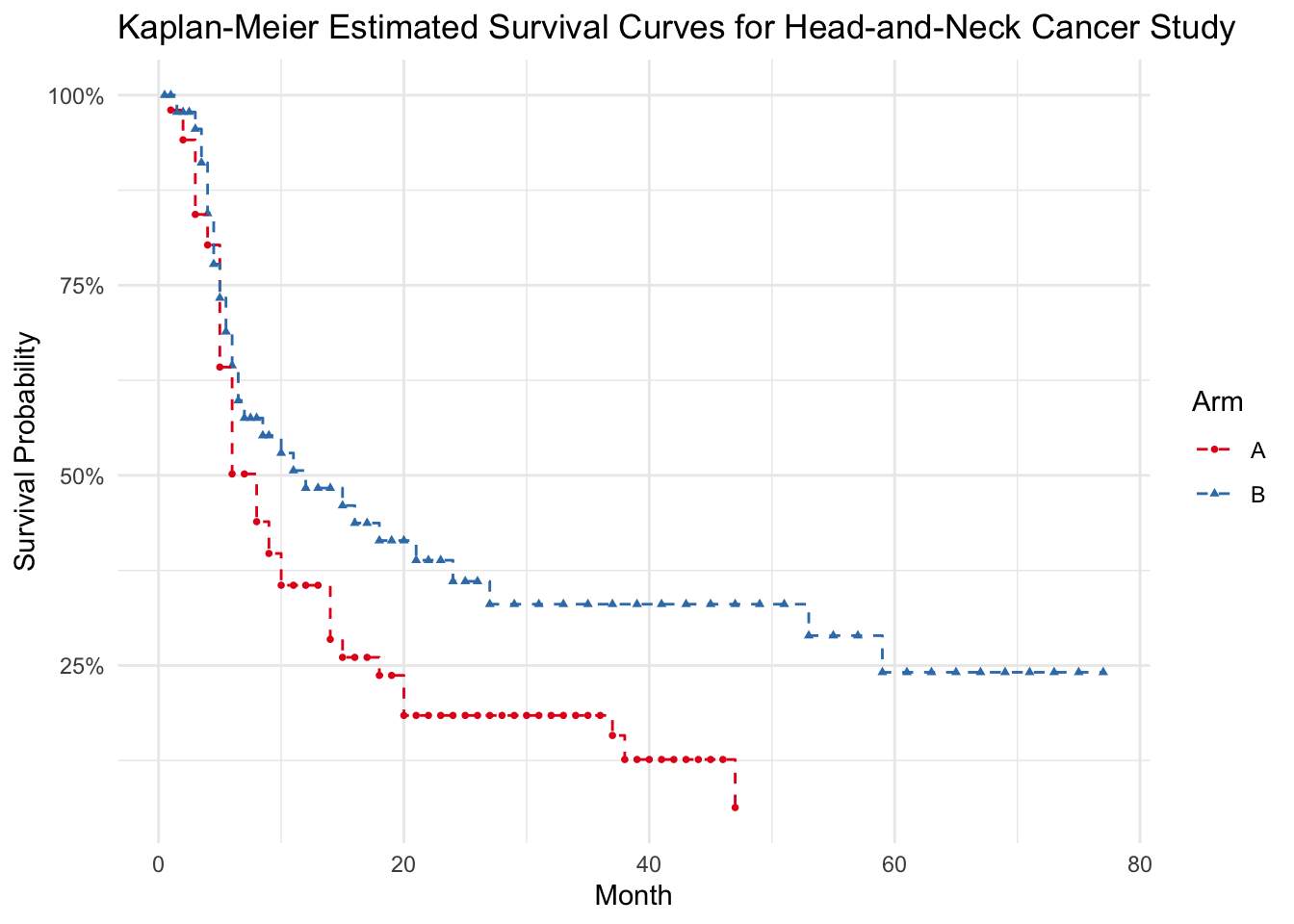
Efron motivates this approach using survival data from a Head-and-Neck cancer study conducted by the Northern California Oncology Group. I’ve extracted this data to replicate the method.

First, let’s show the Kaplan-Meir estimates

library(tidyverse)
library(survival)
library(splines)

source("make_data.R")

sd <- make_data('survival')
sfit <- survfit(Surv(month, event) ~ strata(arm), data=sd, weights = wt)

sfit_tidy <- broom::tidy(sfit) %>% 
             mutate(strata = str_remove(strata, fixed('strata(arm)=')))


base_plot <- sfit_tidy %>% 
  ggplot(aes(time, estimate, color=strata, shape=strata)) + 
  geom_point(size=1) + 
  theme_minimal() + 
  scale_color_brewer(palette = 'Set1') +
  scale_y_continuous(labels = scales::percent) + 
  labs(x='Month', y='Survival Probability', color='Arm', shape='Arm', title='Kaplan-Meier Estimated Survival Curves for Head-and-Neck Cancer Study')


base_plot + 
  geom_step(linetype='dashed')

The intial model presented expands time in the following basis functions

\[ x_i = (1, t_i, (t_i-11)_-^{2}, (t_i-11)_-^{3}) \]

Here, \(t_i\) is the the midpoint between months. This is equivalent to estimating the risk of the outcome between the start of month \(i\) and the start of month \(i+1\). The function \(( z )_- = \min(z, 0)\). This particular expansion allows \(t_i\) to vary as a cubic function before \(t_i=11\), and then as a linear function thereafter.

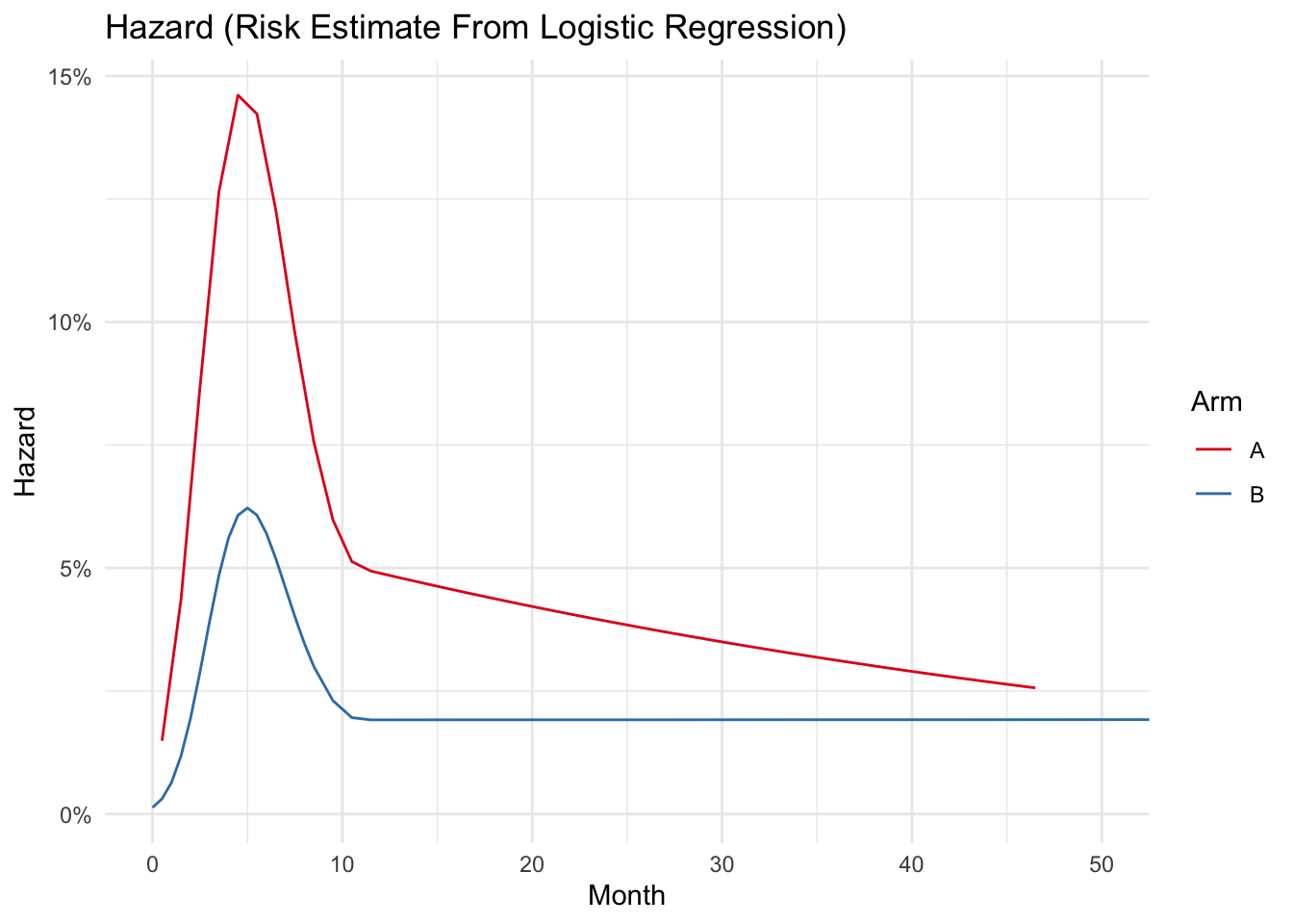
After fitting the model with an interaction by arm (so that the hazards can differ by arm), we can plot the hazards readily ¹.

d <- make_data('logistic') %>% 
     mutate(tm = month - 0.5, 
            txt = as.integer(arm=='A'))


f <- function(x, d) pmin((x), 0)

fit <- glm(cbind(s, n-s) ~ arm * (tm + I(f(tm-11)^2) + I(f(tm-11)^3)),
       data=d, 
       family = binomial())

preds <- d %>% 
  bind_cols(predict(fit, newdata=., se.fit=T)) %>% 
  mutate(
    p = plogis(fit),
    p.low = plogis(fit - 2*se.fit),
    p.high = plogis(fit + 2*se.fit)
  ) %>% 
  group_by(arm) %>% 
  arrange(arm, month) %>% 
  mutate(S = cumprod(1-p),
         S.low = cumprod(1-p.low),
         S.high = cumprod(1-p.high))


preds %>% 
  ggplot(aes(tm, p, color=arm)) +
  geom_line() + 
  coord_cartesian(xlim = c(0, 50)) + 
  theme_minimal() + 
  scale_color_brewer(palette = 'Set1') +
  scale_y_continuous(labels = scales::percent) + 
  labs(x='Month', y='Hazard', color='Arm', shape='Arm', title='Hazard (Risk Estimate From Logistic Regression)')

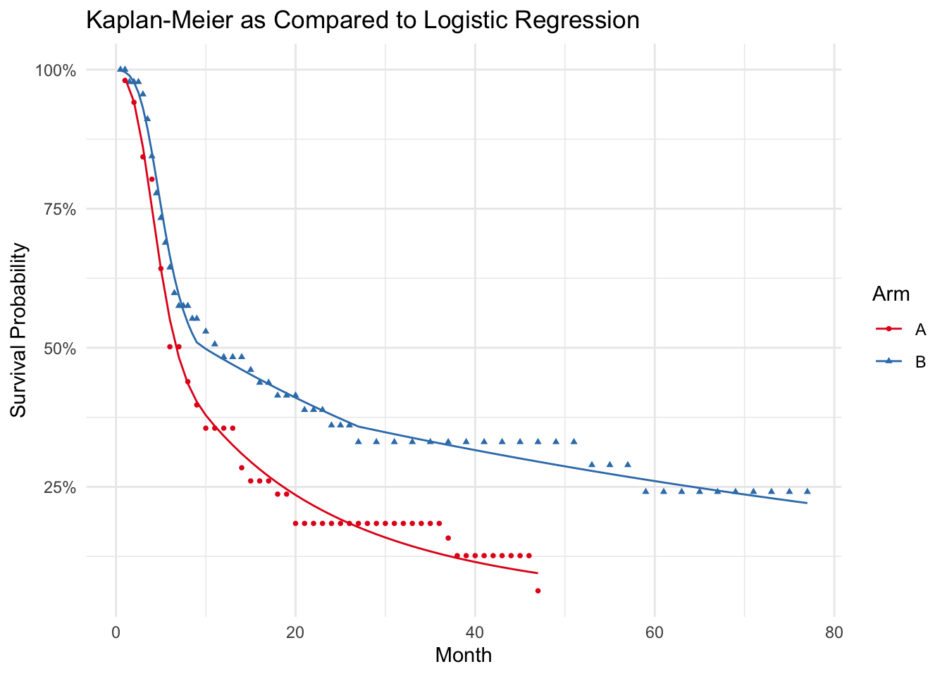
And we can also plot the estimated survival function against the Kaplan Meier to compare.

base_plot + 
  geom_line(data=preds, aes(month, S, color=arm), inherit.aes = F) + 
  labs(title='Kaplan-Meier as Compared to Logistic Regression')

Final Thoughts

Why would we want to parametrically model the hazard when Kaplan-Meir can’t misspecify the hazard? What do we gain from this? In a word: efficiency , at least according to Efron. Additionally, if we are willing to make assumptions about how the hazard evolves into the future (e.g. linearly) then we can use this approach to forecast survival beyond the last observed timepoint.

In his paper, Efron has some notes on computing standard errors for this estimator. Its fairly dense, and I haven’t included confidence intervals here lest I naively compute them. That’s a topic for a future blog post.

Footnotes

1. I Just can’t get the hazard’s to look the same as Figure 2. Might be an error copying over the data.