The Winner’s Curse Is Easy To Understand From This Picture
Author
Demetri Pananos
Published
January 20, 2024
Take a look at the photo below, and it i should be easy to understand why The Winner’s Curse (the general tendency for detected effects to be an over estimate of the truth) is a thing.
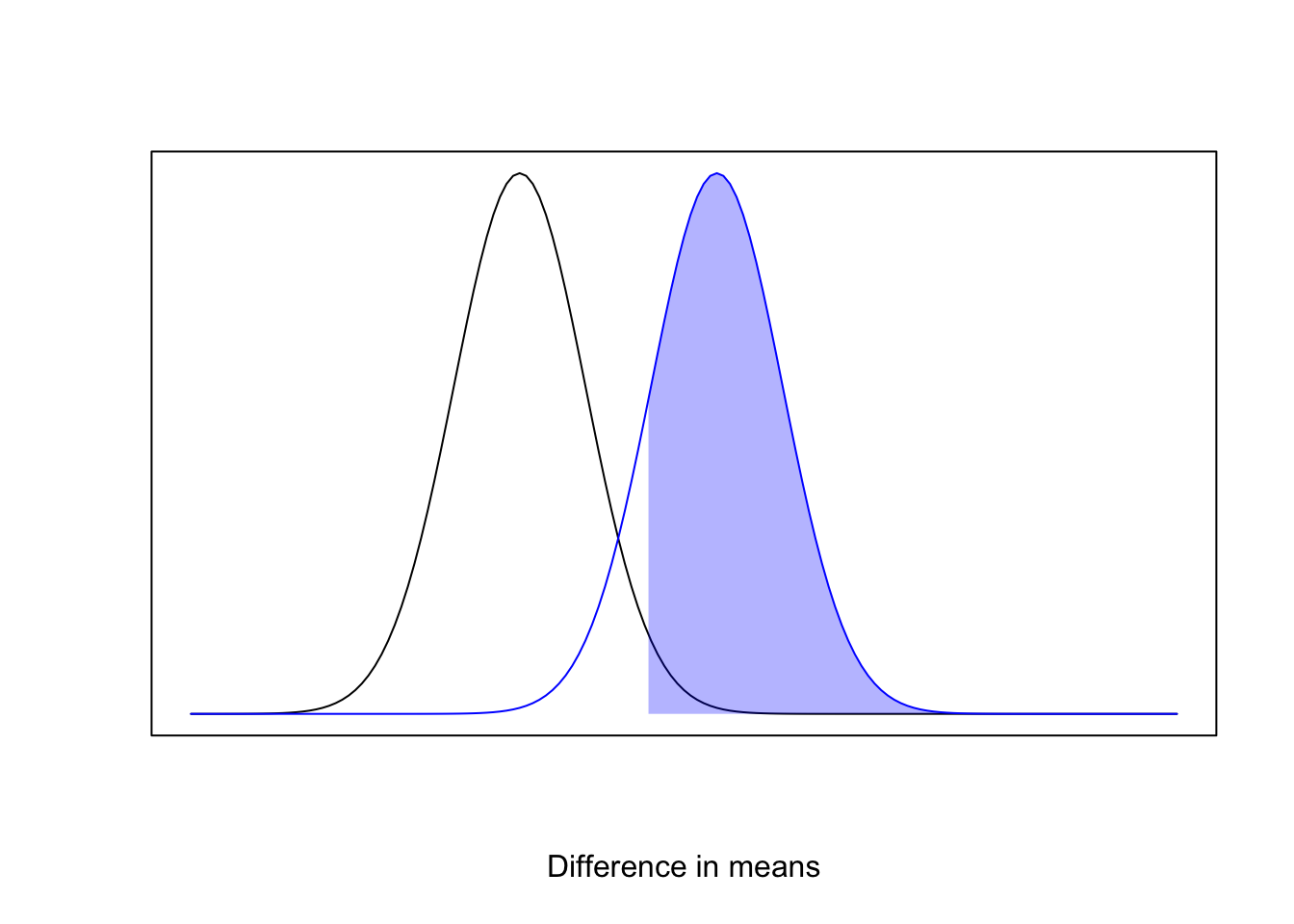
The plot shows our typical setup for a hypothesis test. In black is the sampling distribution of the test statistic for a difference in means under the null, and in blue is the statistic’s sampling distribution under the alternative. The shaded blue region represents the statistical power, and those effect sizes in the shaded region would be considered “statistically significant”.
The shaded blue region defines a lower truncated normal distribution. Were the alternative hypothesis true, and were we to run many experiments to estimate the difference in means, our detected effects would be samples from this distribution. Hence, using those samples to estimate the mean of the alternative distribution would result in a biased estimate of the mean.
The expectation for a lower truncated normal distribution truncated at \(x=a\) is
Here \(\mu\) and \(\sigma\) are the mean and standard deviation of the distribution under the alternative, \(\varphi\) is the standard normal density, \(\Phi\) is the standard normal cumulative distribution. So our estimate of the mean would be biased upwards by \(\sigma \frac{\varphi\left( \frac{a-\mu}{\sigma} \right)}{1 - \Phi\left(\frac{a-\mu}{\sigma}\right)}\). That can be small or large depending on \(\mu\) and \(\sigma\).
Without doing any differentiation to understand where this bias is largest, it should be intutituve from the picture that the bias is small/large when statistical power is large/small.
Hence, estimates from underpowered studies should be met with <fry_squint.jpg>.