You Just Said Something Wrong About Logistic Regression
Author
Demetri Pananos
Published
February 6, 2024
Congratulations, you just said something wrong about logistic regression. That’s OK, logistic regression is hard and we all have to learn/re-learn some things from time to time.
This is a living blog post intended to address some common misconceptions or flat out wrong statements I’ve seen people make about logistic regression.
1 The Coefficients of Logistic Regression are Interpreted as “You’re X Times More Likely to See Y Given Factor Z”.
Wrong! The (exponentiated) coefficients of logistic regression are interpreted as “the odds you see Y given Factor Z are X times larger”.
Phrases like “X times more likely” allude to the the probability of the event. If the probability of getting some event is 10%, and the probability of getting some other event is 20%, then you are 2 times more likely to get the latter event than the former.
This kind of comparison between two probabilities is called “the relative risk” (or risk ratio, or lift, it really depends on where you work). The coefficients of a logistic regression are not risk ratios, nor are they log risk ratios; they are log odds ratios.
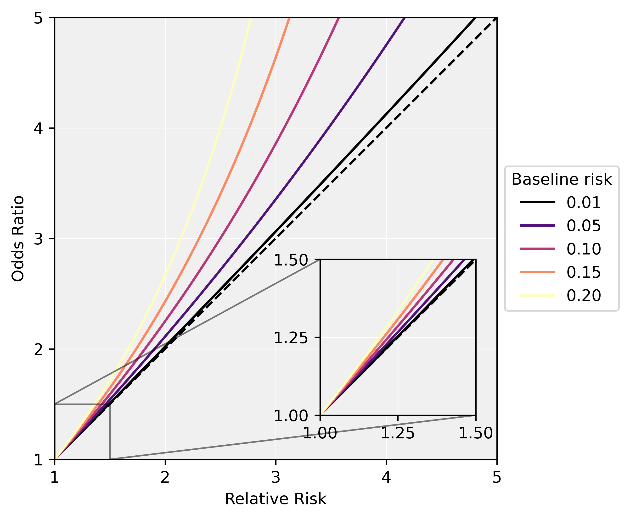
Now, it is actually fine to make this mistake under a few conditions. Namely, when a) the odds ratio is sufficiently small, and/or b) the baseline risk is sufficiently small. You can see this on the plot below which plots the odds ratios and corresponds risk ratios for various baseline risks. On the whole though, you shouldn’t interpret any output from logistic regression as a risk ratio unless you explicitly go out of our way to estimate that quantity.
Code
import numpy as npimport matplotlib.pyplot as pltimport matplotlib.cm as cmfrom mpl_toolkits.axes_grid1.inset_locator import inset_axesp1 = np.array([0.01, 0.05, 0.1, 0.15, 0.20])rr = np.linspace(1, 4.9, 500)fig, ax = plt.subplots(dpi=240)ax.set_aspect('equal')ax.set_xlim(1, 5)ax.set_ylim(1, 5)# Set light gray backgroundax.set_facecolor('#f0f0f0')# Set white grid linesax.grid(color='white', linestyle='-', linewidth=0.5)ax.plot([0, 5], [0, 5], 'k--')cmap = cm.get_cmap('magma')colors = cmap(np.linspace(0, 1, len(p1)))for i, p inenumerate(p1): p2 = rr * p odr = p2 * (1- p) / ((1- p2) * p) ax.plot(rr, odr, label=f"{p:.2f}", color=colors[i])# Move legend outside the plot axis to the rightax.legend(title="Baseline risk", loc='center left', bbox_to_anchor=(1, 0.5))# Set y ticks to [1, 2, 3, 4, 5]ax.set_yticks([1, 2, 3, 4, 5])ax.set_xticks([1, 2, 3, 4, 5])ax.set_xlabel('Relative Risk')ax.set_ylabel('Odds Ratio')# Add zoom inset region axis on the bottom centeraxins = ax.inset_axes( [0.6, 0.1, 0.47*0.75, 0.47*0.75], # Adjusted position xlim=(1, 1.5), ylim=(1, 1.5), xticks=[1, 1.25, 1.5], yticks=[1, 1.25, 1.5])axins.plot([0, 5], [0, 5], 'k--')axins.set_facecolor('#f0f0f0')axins.grid(color='white', linestyle='-', linewidth=0.5)for i, p inenumerate(p1): p2 = rr * p odr = p2 * (1- p) / ((1- p2) * p) axins.plot(rr, odr, label=f"{p:.2f}", color=colors[i])# Use ax.indicate_inset_zoom to draw a rectangle around the zoomed-in regionax.indicate_inset_zoom(axins, edgecolor="black")plt.show()
How the relative risk and odds ratio differ for various baseline risks. For each basline risk, we can compute the associated probabiltity given the relative risk. Given that probability, we can also compute the odds ratio.