Gradient Descent with ODEs

Gradient descent usually isn’t used to fit Ordinary Differential Equations (ODEs) to data (at least, that isn’t how the Applied Mathematics departments to which I have been a part have done it). Nevertheless, that doesn’t mean that it can’t be done. For some of my recent GSoC work, I’ve been investigating how to compute gradients of solutions to ODEs without access to the solution’s analytical form. In this blog post, I describe how these gradients can be computed and how they can be used to fit ODEs to synchronous data with gradient descent.

Up To Speed With ODEs

I realize not everyone might have studied ODEs. Here is everything you need to know:

A differential equation relates an unknown function \(y \in \mathbb{R}^n\) to it’s own derivative through a function \(f: \mathbb{R}^n \times \mathbb{R} \times \mathbb{R}^m \rightarrow \mathbb{R}^n\), which also depends on time \(t \in \mathbb{R}\) and possibly a set of parameters \(\theta \in \mathbb{R}^m\). We usually write ODEs as

\[y' = f(y,t,\theta) \quad y(t_0) = y_0\]

Here, we refer to the vector \(y\) as “the system”, since the ODE above really defines a system of equations. The problem is usually equipped with an initial state of the system \(y(t_0) = y_0\) from which the system evolves forward in \(t\). Solutions to ODEs in analytic form are often very hard if not impossible, so most of the time we just numerically approximate the solution. It doesn’t matter how this is done because numerical integration is not the point of this post. If you’re interested, look up the class of Runge-Kutta methods.

Computing Gradients for ODEs

In this section, I’m going to be using derivative notation rather than \(\nabla\) for gradients. I think it is less ambiguous.

If we want to fit an ODE model to data by minimizing some loss function \(\mathcal{L}\), then gradient descent looks like

\[ \theta_{n+1} = \theta_n - \alpha \dfrac{\partial \mathcal{L}}{\partial \theta} \]

In order to compute the gradient of the loss, we need the gradient of the solution, \(y\), with respect to \(\theta\). The gradient of the solution is the hard part here because it can not be computed (a) analytically (because analytic solutions are hard AF), or (b) through automatic differentiation without differentiating through the numerical integration of our ODE (which seems computationally wasteful).

Thankfully, years of research into ODEs yields a way to do this (that is not the adjoint method. Surprise! You thought I was going to say the adjoint method didn’t you?). Forward mode sensitivity analysis calculates gradients by extending the ODE system to include the following equations:

\[ \dfrac{d}{dt}\left( \dfrac{\partial y}{\partial \theta} \right) = \mathcal{J}_f \dfrac{\partial y}{\partial \theta} +\dfrac{\partial f}{\partial \theta} \]

Here, \(\mathcal{J}\) is the Jacobian of \(f\) with respect to \(y\). The forward sensitivity analysis is just another differential equation (see how it relates the derivative of the unknown \(\partial y / \partial \theta\) to itself?)! In order to compute the gradient of \(y\) with respect to \(\theta\) at time \(t_i\), we compute

\[ \dfrac{\partial y}{\partial \theta} = \int_{t_0}^{t_i} \mathcal{J}_f \dfrac{\partial y}{\partial \theta} + \dfrac{\partial f}{\partial \theta} \, dt \]

I know this looks scary, but since forward mode sensitivities are just ODEs, we actually just get this from what we can consider to be a black box

\[\dfrac{\partial y}{\partial \theta} = \operatorname{BlackBox}(f(y,t,\theta), t_0, y_0, \theta)\]

So now that we have our gradient in hand, we can use the chain rule to write

\[\dfrac{\partial \mathcal{L}}{\partial \theta} =\dfrac{\partial \mathcal{L}}{\partial y} \dfrac{\partial y}{\partial \theta} \]

We can use automatic differentiation to compute \(\dfrac{\partial \mathcal{L}}{\partial y}\).

OK, so that is some math (interesting to me, maybe not so much to you). Let’s actually implement this in python.

Gradient Descent for the SIR Model

The SIR model is a set of differential equations which govern how a disease spreads through a homogeneously mixed closed populations. I could write an entire thesis on this model and its various extensions (in fact, I have), so I’ll let you read about those on your free time.

The system, shown below, is parameterized by a single parameter:

\[ \dfrac{dS}{dt} = -\theta SI \quad S(0) = 0.99 \]

\[ \dfrac{dI}{dt} = \theta SI - I \quad I(0) = 0.01 \]

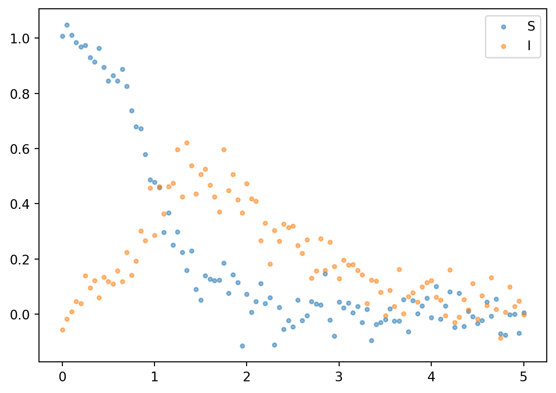
Let’s define the system, the appropriate derivatives, generate some observations and fit \(\theta\) using gradient descent. Here si what you’ll need to get started:

import autograd
from autograd.builtins import tuple
import autograd.numpy as np

#Import ode solver and rename as BlackBox for consistency with blog
from scipy.integrate import odeint as BlackBox
import matplotlib.pyplot as plt

Let’s then define the ODE system

def f(y,t,theta):
    '''Function describing dynamics of the system'''
    S,I = y
    ds = -theta*S*I
    di = theta*S*I - I

    return np.array([ds,di])

and take appropriate derivatives

#Jacobian wrt y
J = autograd.jacobian(f,argnum=0)
#Gradient wrt theta
grad_f_theta = autograd.jacobian(f,argnum=2)

Next, we’ll define the augmented system (that is, the ODE plus the sensitivities).

def ODESYS(Y,t,theta):

    #Y will be length 4.
    #Y[0], Y[1] are the ODEs
    #Y[2], Y[3] are the sensitivities

    #ODE
    dy_dt = f(Y[0:2],t,theta)
    #Sensitivities
    grad_y_theta = J(Y[:2],t,theta)@Y[-2::] + grad_f_theta(Y[:2],t,theta)

    return np.concatenate([dy_dt,grad_y_theta])

We’ll optimize the \(L_2\) norm of the error

def Cost(y_obs):
    def cost(Y):
        '''Squared Error Loss'''
        n = y_obs.shape[0]
        err = np.linalg.norm(y_obs - Y, 2, axis = 1)

        return np.sum(err)/n

    return cost

Create some observations from which to fit

np.random.seed(19920908)
## Generate Data
#Initial Condition
Y0 = np.array([0.99,0.01, 0.0, 0.0])
#Space to compute solutions
t = np.linspace(0,5,101)
#True param value
theta = 5.5

sol = BlackBox(ODESYS, y0 = Y0, t = t, args = tuple([theta]))

#Corupt the observations with noise
y_obs = sol[:,:2] + np.random.normal(0,0.05,size = sol[:,:2].shape)

plt.scatter(t,y_obs[:,0], marker = '.', alpha = 0.5, label = 'S')
plt.scatter(t,y_obs[:,1], marker = '.', alpha = 0.5, label = 'I')


plt.legend()

<matplotlib.legend.Legend at 0x7f8e9d0b3d30>

Perform Gradient Descent

theta_iter = 1.5
cost = Cost(y_obs[:,:2])
grad_C = autograd.grad(cost)

maxiter = 100
learning_rate = 1 #Big steps
for i in range(maxiter):

    sol = BlackBox(ODESYS,y0 = Y0, t = t, args = tuple([theta_iter]))

    Y = sol[:,:2]

    theta_iter -=learning_rate*(grad_C(Y)*sol[:,-2:]).sum()

    if i%10==0:
        print("Theta estimate: ", theta_iter)

Theta estimate:  1.697027594337629

Theta estimate:  3.9189060278370365

Theta estimate:  4.810038385538704

Theta estimate:  5.251499985105974

Theta estimate:  5.427206219478129

Theta estimate:  5.46957706068474

Theta estimate:  5.47744643541383

Theta estimate:  5.4792194685272095

Theta estimate:  5.479636817124458

Theta estimate:  5.47973599525063

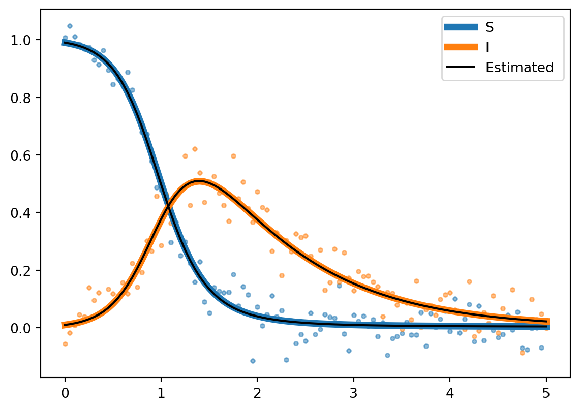
And lastly, compare our fitted curves to the true curves

sol = BlackBox(ODESYS, y0 = Y0, t = t, args = tuple([theta_iter]))
true_sol = BlackBox(ODESYS, y0 = Y0, t = t, args = tuple([theta]))


plt.plot(t,sol[:,0], label = 'S', color = 'C0', linewidth = 5)
plt.plot(t,sol[:,1], label = 'I', color = 'C1', linewidth = 5)

plt.scatter(t,y_obs[:,0], marker = '.', alpha = 0.5)
plt.scatter(t,y_obs[:,1], marker = '.', alpha = 0.5)


plt.plot(t,true_sol[:,0], label = 'Estimated ', color = 'k')
plt.plot(t,true_sol[:,1], color = 'k')

plt.legend()

<matplotlib.legend.Legend at 0x7f8e9de4e5e0>

Conclusions

Fitting ODEs via gradient descent is possible, and not as complicated as I had initially thought. There are still some relaxations to be explored. Namely: what happens if we have observations at time \(t_i\) for one part of the system but not the other? How does this scale as we add more parameters to the model? Can we speed up gradient descent some how (because it takes too long to converge as it is, hence the maxiter variable). In any case, this was an interesting, yet related, divergence from my GSoC work. I hope you learned something.