I wrote an answer to a question about sequences of coin flips a couple days back that I was quite chuffed with. In short, the question asked for statistical ways to determine if a sequence of coin flips was from an unbiased coin or a human trying to appear random. The resulting model turned into a fun game on twitter centered around determining if people who follow me could simulate a sequence of coin flips that looked random (without using a real RNG, or some funny workaround. I have a lot of faith in my twitter followers…maybe too much).
Anyway, then I thought “I should fit a hierarchical model to this data”. So that’s what I’m doing
Initial Model
To understand the hierarchical model, we first need to understand the model I initially built. Let me give you a quick rundown on that.
Let \(S\) be a sequence of bernoulli experiments so that \(S_i\) is either 1 or a 0 (a heads or a tails if you wish). The question I answered concerns detecting if a given sequence \(S\) could have been created by a human (or by a non-random process posing as random). I interpreted that as a call to estimate the lag-1 autocorrelation of the flips. The hypothesis being that humans probably perceive long streaks of one outcome or the other as signs of non-randomness and will intentionally switch the outcome if they feel the run is too long. I initially chose a Bayesian approach because I’m a glutton for punishment and someone else already gave a pretty good answer.
The model is quite straight forward to write down. Let \(\rho\) be the correlation between \(S_i\) and \(S_{i+1}\), and let \(q\) be the expected number of heads in the sequence. We can write down the conditional probabilities that we see a 0/1 given the last element in the sequence was a 1/0. Those conditional probabilities are derived here and they are…
\[ P(1 \vert 1) = q + \rho(1-q) \]
\[ P(1 \vert 0) = q(1-\rho) \]
\[ P(0 \vert 1) = (1-q)(1-\rho) \]
\[ P(0 \vert 0) = 1 - q + \rho \cdot q \]
The trick is to then count the subsequences of (1, 1), (1, 0), (0, 1), and (0, 0). Let \(p_{i\vert j} = P(i \vert j)\). We can then consider the count of each subsequence as multinomial
\[ y \sim \mbox{Multinomial}(\theta) \>. \]
Here, \(\theta\) is the multinomial parameter, wherein each element is \(\theta = [p_{1 \vert 1}, p_{1\vert 0}, p_{0 \vert 1}, p_{0\vert 0}]\). Equip this with a uniform prior on both \(\rho\) and \(q\) and you’ve got yourself a model.
The Stan Code
The Stan code for this model is quite easy to understand. The data block will consist of the counts of each type of subsequence. We can then concatenate those counts into an int of length 4 via the transformed data block. The concatenated counts will be what we pass to the multinomial likelihood.
data{
  int y_1_1; //number of concurrent 1s
  int y_0_1; //number of 0,1 occurences
  int y_1_0; //number of 1,0 occurences
  int y_0_0; //number of concurrent 0s
}
transformed data{
    int y[4] = {y_1_1, y_0_1, y_1_0, y_0_0};
}
The only parameters we are interested in estimating are the autocorrelation rho and the coin’s bias q.
We can derive the probabilities we need via the equations above, and that is a job for the transformed parameters block. We can then concatenate the conditional probabilities into a simplex data type object, theta to pass to the multinomial likelihood. Be careful though, we need to multiply theta by 0.5 since we are working with conditional probabilities. Note \(p_{1\vert 1} + p_{0 \vert 1 } + p_{1\vert 0} + p_{0 \vert 0 } = 2\), hence the scaling factor.
With the model written down, all we need to do is add some python code to create the counts of each subsequence and then run the stan model. Here is teh python code I used to create the response tweets for that game I ran on twitter.
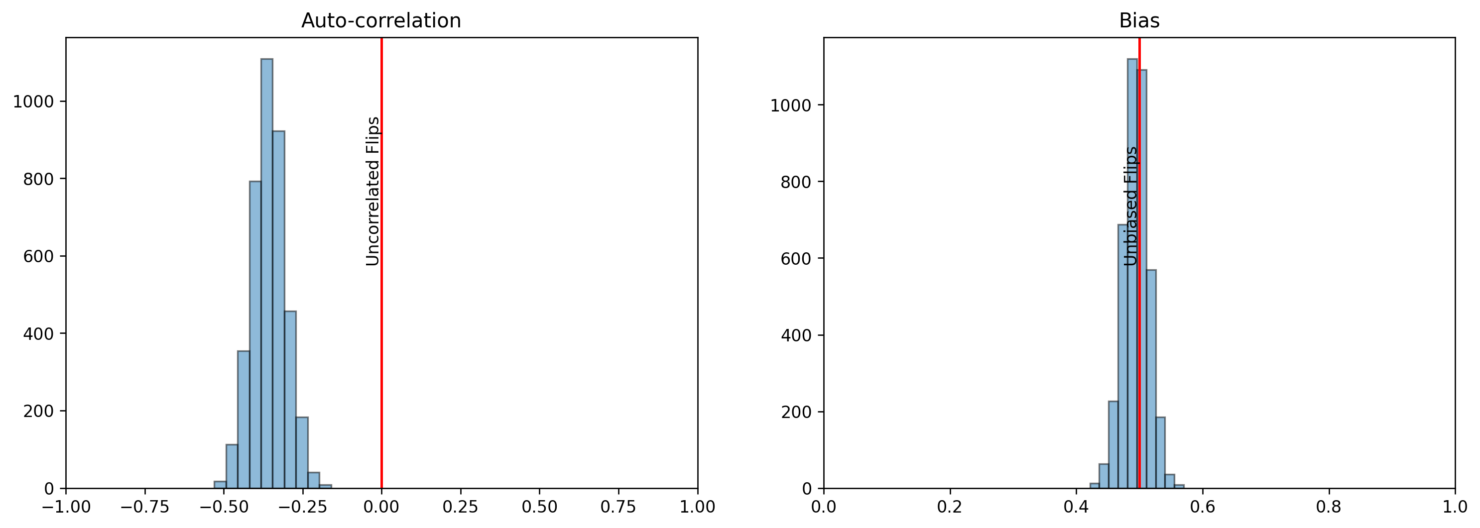
import cmdstanpyimport matplotlib.pyplot as plty_1_1 =0# count of (1, 1)y_0_0 =0# count of (0, 0)y_0_1 =0# count of (0, 1)y_1_0 =0# count of (1, 0)sequence =list('TTHHTHTTHTTTHTTTHTTTHTTHTHHTHHTHTHHTTTHHTHTHTTHTHHTTHTHHTHTTTHHTTHHTTHHHTHHTHTTHTHTTHHTHHHTTHTHTTTHHTTHTHTHTHTHTTHTHTHHHTTHTHTHHTHHHTHTHTTHTTHHTHTHTHTTHHTTHTHTTHHHTHTHTHTTHTTHHTTHTHHTHHHTTHHTHTTHTHTHTHTHTHTHHHTHTHTHTHHTHHTHTHTTHTTTHHTHTTTHTHHTHHHHTTTHHTHTHTHTHHHTTHHTHTTTHTHHTHTHTHHTHTTHTTHTHHTHTHTTT'.upper())# Do a rolling window trick I saw somewhere on twitter.# This implements a rollowing window of 2# In python 3.10, this would be a great use case for matchfor pairs inzip(sequence[:-1], sequence[1:]):if pairs == ('H','H'): y_1_1 +=1elif pairs == ('T','H'): y_0_1 +=1elif pairs == ('H', 'T'): y_1_0 +=1else: y_0_0 +=1# Write the stan model as a string. We will then write it to a filestan_code ='''data{ int y_1_1; //number of concurrent 1s int y_0_1; //number of 0,1 occurences int y_1_0; //number of 1,0 occurences int y_0_0; //number of concurrent 0s}transformed data{ int y[4] = {y_1_1, y_0_1, y_1_0, y_0_0};}parameters{ real<lower=-1, upper=1> rho; real<lower=0, upper=1> q;}transformed parameters{ real<lower=0, upper=1> prob_1_1 = q + rho*(1-q); real<lower=0, upper=1> prob_0_1 = (1-q)*(1-rho); real<lower=0, upper=1> prob_1_0 = q*(1-rho); real<lower=0, upper=1> prob_0_0 = 1 - q + rho*q; simplex[4] theta = 0.5*[prob_1_1, prob_0_1, prob_1_0, prob_0_0 ]';}model{ q ~ beta(1, 1); rho ~ uniform(-1, 1); y ~ multinomial(theta);}generated quantities{ vector[300] yppc; yppc[1] = bernoulli_rng(q); for(i in 2:300){ if(yppc[i-1]==1){ yppc[i] = bernoulli_rng(prob_1_1); } else{ yppc[i] = bernoulli_rng(prob_1_0); } }}'''# Write the model to a temp filewithopen('model_file.stan', 'w') as model_file: model_file.write(stan_code)# Compile the modelmodel = cmdstanpy.CmdStanModel(stan_file='model_file.stan')# data to pass to Standata =dict(y_1_1 = y_1_1, y_0_0 = y_0_0, y_0_1 = y_0_1, y_1_0 = y_1_0)# Plotting stuff.fig, ax = plt.subplots(dpi =120, ncols=2, figsize = (15, 5))ax[0].set_title('Auto-correlation')ax[1].set_title('Bias')ax[0].set_xlim(-1, 1)ax[1].set_xlim(0, 1)ax[0].axvline(0, color ='red')ax[1].axvline(0.5, color ='red')ax[0].annotate('Uncorrelated Flips', xy=(0.475, 0.5), xycoords='axes fraction', rotation =90)ax[1].annotate('Unbiased Flips', xy=(0.475, 0.5), xycoords='axes fraction', rotation =90)# MCMC go brrrrfit = model.sample(data)ax[0].hist(fit.stan_variable('rho'), edgecolor='k', alpha =0.5)ax[1].hist(fit.stan_variable('q'), edgecolor='k', alpha =0.5)autocorr = fit.stan_variable('rho').mean()bias = fit.stan_variable('q').mean()tweet =f"Your flips have an expected correlation of {autocorr:.2f} and your coin's bias is about {bias:.2f}"print(f"Your sequence was {''.join(sequence)}")print(tweet)
INFO:cmdstanpy:compiling stan file /Users/demetri/Documents/dpananos.github.io/posts/2022-05-07-flippin/model_file.stan to exe file /Users/demetri/Documents/dpananos.github.io/posts/2022-05-07-flippin/model_file
INFO:cmdstanpy:compiled model executable: /Users/demetri/Documents/dpananos.github.io/posts/2022-05-07-flippin/model_file
WARNING:cmdstanpy:Stan compiler has produced 1 warnings:
WARNING:cmdstanpy:
--- Translating Stan model to C++ code ---
bin/stanc  --o=/Users/demetri/Documents/dpananos.github.io/posts/2022-05-07-flippin/model_file.hpp /Users/demetri/Documents/dpananos.github.io/posts/2022-05-07-flippin/model_file.stan
Warning in '/Users/demetri/Documents/dpananos.github.io/posts/2022-05-07-flippin/model_file.stan', line 11, column 4: Declaration
    of arrays by placing brackets after a variable name is deprecated and
    will be removed in Stan 2.32.0. Instead use the array keyword before the
    type. This can be changed automatically using the auto-format flag to
    stanc

--- Compiling, linking C++ code ---
clang++ -std=c++1y -Wno-unknown-warning-option -Wno-tautological-compare -Wno-sign-compare -D_REENTRANT -Wno-ignored-attributes      -I stan/lib/stan_math/lib/tbb_2020.3/include    -O3 -I src -I stan/src -I lib/rapidjson_1.1.0/ -I lib/CLI11-1.9.1/ -I stan/lib/stan_math/ -I stan/lib/stan_math/lib/eigen_3.3.9 -I stan/lib/stan_math/lib/boost_1.75.0 -I stan/lib/stan_math/lib/sundials_6.0.0/include -I stan/lib/stan_math/lib/sundials_6.0.0/src/sundials    -DBOOST_DISABLE_ASSERTS          -c -include-pch stan/src/stan/model/model_header.hpp.gch -x c++ -o /Users/demetri/Documents/dpananos.github.io/posts/2022-05-07-flippin/model_file.o /Users/demetri/Documents/dpananos.github.io/posts/2022-05-07-flippin/model_file.hpp
clang++ -std=c++1y -Wno-unknown-warning-option -Wno-tautological-compare -Wno-sign-compare -D_REENTRANT -Wno-ignored-attributes      -I stan/lib/stan_math/lib/tbb_2020.3/include    -O3 -I src -I stan/src -I lib/rapidjson_1.1.0/ -I lib/CLI11-1.9.1/ -I stan/lib/stan_math/ -I stan/lib/stan_math/lib/eigen_3.3.9 -I stan/lib/stan_math/lib/boost_1.75.0 -I stan/lib/stan_math/lib/sundials_6.0.0/include -I stan/lib/stan_math/lib/sundials_6.0.0/src/sundials    -DBOOST_DISABLE_ASSERTS                -Wl,-L,"/Users/demetri/.cmdstan/cmdstan-2.29.2/stan/lib/stan_math/lib/tbb" -Wl,-rpath,"/Users/demetri/.cmdstan/cmdstan-2.29.2/stan/lib/stan_math/lib/tbb"      /Users/demetri/Documents/dpananos.github.io/posts/2022-05-07-flippin/model_file.o src/cmdstan/main.o        -Wl,-L,"/Users/demetri/.cmdstan/cmdstan-2.29.2/stan/lib/stan_math/lib/tbb" -Wl,-rpath,"/Users/demetri/.cmdstan/cmdstan-2.29.2/stan/lib/stan_math/lib/tbb"   stan/lib/stan_math/lib/sundials_6.0.0/lib/libsundials_nvecserial.a stan/lib/stan_math/lib/sundials_6.0.0/lib/libsundials_cvodes.a stan/lib/stan_math/lib/sundials_6.0.0/lib/libsundials_idas.a stan/lib/stan_math/lib/sundials_6.0.0/lib/libsundials_kinsol.a  stan/lib/stan_math/lib/tbb/libtbb.dylib stan/lib/stan_math/lib/tbb/libtbbmalloc.dylib stan/lib/stan_math/lib/tbb/libtbbmalloc_proxy.dylib -o /Users/demetri/Documents/dpananos.github.io/posts/2022-05-07-flippin/model_file
rm -f /Users/demetri/Documents/dpananos.github.io/posts/2022-05-07-flippin/model_file.o
INFO:cmdstanpy:CmdStan start processing
INFO:cmdstanpy:CmdStan done processing.
Your sequence was TTHHTHTTHTTTHTTTHTTTHTTHTHHTHHTHTHHTTTHHTHTHTTHTHHTTHTHHTHTTTHHTTHHTTHHHTHHTHTTHTHTTHHTHHHTTHTHTTTHHTTHTHTHTHTHTTHTHTHHHTTHTHTHHTHHHTHTHTTHTTHHTHTHTHTTHHTTHTHTTHHHTHTHTHTTHTTHHTTHTHHTHHHTTHHTHTTHTHTHTHTHTHTHHHTHTHTHTHHTHHTHTHTTHTTTHHTHTTTHTHHTHHHHTTTHHTHTHTHTHHHTTHHTHTTTHTHHTHTHTHHTHTTHTTHTHHTHTHTTT
Your flips have an expected correlation of -0.36 and your coin's bias is about 0.49
Stack Layers…Wait, That’s a Deep Learning Thing
Now it’s time to write a hierarchical model, and for that we need to be a little more careful. I initially thought I could just put priors on the population level autocorrelation and bias, but I quickly ran into a problem there, which I will illustrate below.
Suppose the coin’s bias is 0 (we always get tails). Could the autocorrelation be -1? No, it couldn’t be, because that would mean our next flip would have to be a 1, but the coin’s bias is 0! This illustrates some nuance to the problem I had failed to consider but luckily did not suffer from. The autocorrelation for two binary random variables, \(X, Y\), is defined as
\[ \rho = \dfrac{\alpha - q}{q(1-q)} \]
Where \(E(XY) = \alpha\). You see, \(\alpha\) can only be so big depending on the value of \(q\), and if you place uniform priors on both \(\rho\) and \(q\) you can quickly get conditional probabilities outside the unit interval. That’s exactly what happened, and I was banging my head against the wall for a night trying to figure out the bounds on \(\rho\) given \(q\) and it quickly became a mess.
There is another way. Rather than place priors on \(\rho\) and \(q\), we could place priors on the multinomial parameter and then do algebra (two equations, two unknowns) to find out expressions for \(q\) and \(\rho\) in terms of \(p_{1\vert1}\) and \(p_{1\vert0}\). This isn’t ideal, because I have very good prior information on what \(\rho\) and \(q\) should be, not on what \(\theta\) should be. Whatever, let’s proceed and see how our priors look like with a prior predictive check.
The model is actually simpler to write in Stan than the previous model. We will place a Dirichlet prior on the multinomial parameters (one for each person who responded with a sequence), and then each sequence is multinomial with that multinomial parameter.
\[ \theta_j \sim \mbox{Dirichlet}(\alpha) \]
\[ y_j \sim \mbox{Multinomial}(\theta_j) \]
The quantities we care about can be expressed in terms of \(\theta\)
data{

    int N; //How many sequences do we have
    int y[N, 4]; // matrix of counts of co-occurences of (1,1), (1,0), (0, 1), (0,0)
    int do_sample; // Flag to do a prior predictive check

}
parameters{
    vector<lower=0>[4] a;
    simplex[4] theta[N];
}
model{

  a ~ cauchy(0, 2.5);

  if(do_sample>0){
      for(i in 1:N){
          theta[i] ~ dirichlet(a);
          y[i] ~ multinomial(theta[i]);
      }
    }

}
generated quantities{

    vector[4] theta_ppc = dirichlet_rng(a);
    real rho = theta_ppc[1] - theta_ppc[2];
    real q = 2* theta_ppc[2]/(1 - theta_ppc[1] + theta_ppc[2]);

    real yppc[N, 4];

    for(i in 1:N){
        yppc[i] = multinomial_rng(theta[i], sum(y[i]));
    }
}
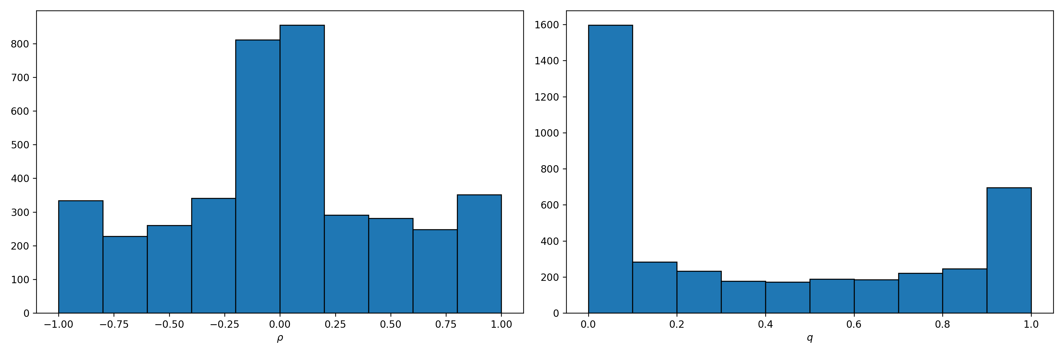
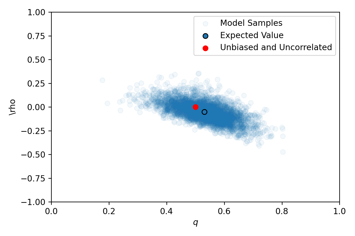
Shown below are the priors for the autocorrelation and bias based on the priors I’ve used. They are a little too uncertain for my liking. Humans are pretty smart, and I don’t expect for the population average bias to be very far from 0.5. I would prefer that the prior for \(q\) be very tightly centered around 0.5, and that the prior for \(\rho\) be tightly centered on 0, but that’s life. The model runs the 76 sequences in about 12 seconds (4 chains, 1000 warmups, 1000 samples) and diagnostics don’t indicate any pathological behavior. Let’s look at the joint posterior.
(a) Priors
(b) Posteriors
Figure 1: Prior and Posterior distributions for the model.
The take home here is that the sequences are largely consistent with an unbiased and uncorrelated coin. The expected correlation is negative (-0.05) meaning humans are more likely to switch from heads to tails, or tails to heads, and the expected bias is 0.53 meaning people seem to favor heads for some reason. The results are largely unsurprising, and I really wish I could place priors on \(\rho\) and \(q\) directly so that my model really does reflect the state of my knowledge, but this is good enough for now.
Conclusion
I’ve been thinking about this problem for a while after I watched a talk by Gelman where he mentioned estimating the autocorrelation between bernoulli experiments in passing (he was talking about model criticism and offering examples of other things to check our model with). I’m moderately happy with the hierarchical model, and the results make a lot of sense. Humans are pretty smart, and we have an intuitive sense for what random looks like. I’m willing to bet that if people submitted longer sequences, we would have a more precise estimate of the bias/correlation.
One thing I’ve shirked is really detailed model criticism, though I have an idea of how I would do that. In that answer on cross validated, COOLSerdash posts a REALLY COOL way to visualize the sequence data. They plot the number of runs (sequences of consecutive heads or tails) against the longest run in the sequence. I think this would make for an excellent way to check that our model has learned the correct autocorrelation for each individual who participated in the game (though I think the sequences were too short to have a precise estimate).