Sometimes we run AB tests where engaging with the treatment (and hence being treated) is optional. Since assignment to treatment is random, we can use the randomization as an instrumental variable (assuming there is a strong correlation between the instrument and the treatment, and that there are no backdoor paths between randomization and the final outcome).

There are a few libraries to do estimate the LATE from an instrumental variable. However, none of them report a causal risk ratio, which is usually our choice of causal contrast for better or worse.

In this post, I’m putting together some much appreciated advice from @guilhermejd1 and dimitry on cross validated on how to estimate a causal risk ratio in a randomized experiment with one sided non-compliance. I’ll first demonstrate how to do this with a simulation where we will actually have potential outcomes with which to compare. Then, I’ll apply this approach to a real experiment I helped run at Zapier.

Simulation

Let \(A\) be a binary indicator for assignment to treatment (1) or control (0). Let \(d_j^a\) be the potential outcome for engaging with the treatment under treatment \(A=a\) for user \(j\). Due to construction of the experiment, \(d_j^0 = 0 \forall j\) because users in control can not engage in the treatment by design. Dimitry writes

“This is different than the typical experiment in labor economics, where people can take up job training somewhere else even if they are in the control group”.

This means that we have two types of users in treatment group: \(d_j^1 = 1\) is a “complier” and \(d_j^1 = 0\) is a “never taker”. If our outcome is \(y\), then LATE is the ATE for compliers and is also the ATT.

Let’s set up a simulation. Here are some details:

\(A\) is decided by a coinflip (i.e. bernoulli with probability of success 0.5)
There is an unmeasured confounder \(w\), which is also distributed in the population via a coinflip.
The confounder and the treatment effect the probability of engaging with the treatment (being a complier). \(P\left(d_j^1 = 1 \mid A=1, w\right) = 0.4 - 0.2w\). Because of the one sided compliance, \(P(d_j^0=1) = 0\).
Probability of the outcome is \(P\left( y^a_j=1 \mid d^{a}_j, w \right) = 0.1 + 0.5w + 0.1d_j^{a}\). So the instrument only effects the outcome through compliance.

Let’s simuilate this in R

library(tidyverse)
library(kableExtra)
my_blue <- rgb(45/250, 62/250, 80/250, 1)
theme_set(theme_classic()) 

update_geom_defaults("point",   list(fill = my_blue, shape=21, color = 'black'))

set.seed(0)
N<- as.integer(1e6) # Lots of precision
A <- rbinom(N, 1, 0.5)
w <- rbinom(N, 1, 0.5)

# Potential outcomes
d_0 <- 0
d_1 <- rbinom(N, 1, 0.3 - 0.2*w + 0.1*A)
y_0 <- rbinom(N, 1, 0.1 + 0.5*w)
y_1 <- rbinom(N, 1, 0.1 + 0.5*w + 0.1*d_1)

# and now the observed data via switching equation
y <- A*y_1 + (1-A)*y_0
d <- A*d_1 + (1-A)*d_0
complier <- d==1

From our setup, \(LATE = 0.1\). Let’s compute that from our potential outcomes and estimate it using \(A\) as an instrument.

sample_late <- mean(y_1[d_1==1]) - mean(y_0[d_1==1])
est_late <- cov(y, A)/cov(d, A)

True LATE	Sample LATE	IV Estimate of LATE
0.1	0.101	0.103

True LATE, sample LATE, and estimated LATE. All 3 agree to within 3 decimal places and any differences are just sampling variability.

Estimating The Causal Risk Ratio

In order to compute the causal risk ratio we need two quantities:

An estimate of \(E[y^1_j \mid d^1]\), and
An estimate of \(E[y^0_j \mid d^1]\).

\(E[y^1_j \mid d^1]\) is easy to estimate; just compute the average outcome of those users in treatment who engaged with the treatment. Now because \(LATE = E[y^1_j \mid d^1] - E[y^0_j \mid d^1]\), the second estimate we need is obtained from some algebra.

# Estimate from the data
E_y1 <- mean(y[d==1])
E_y0 <- E_y1 - est_late # use the estimate, not the truth

E_y1/E_y0

[1] 1.389267

Let’s compare this to the true estimate of the causal risk ratio using potential outcomes

mean(y_1[complier])/mean(y_0[complier])

[1] 1.381259

Which is pretty damn close.

A Real Example

We ran an experiment where users could optionally watch a video. The video was intended to drive some other metric \(y\). Here are the results from the experiment.

Characteristic	Overall, N = 10,119¹	Complied, N = 219¹	Never Taker, N = 9,900¹
Y
0	5,932.0 (58.6%)	145.0 (66.2%)	5,787.0 (58.5%)
1	4,187.0 (41.4%)	74.0 (33.8%)	4,113.0 (41.5%)
Treatment
Control	5,083.0 (50.2%)	0.0 (0.0%)	5,083.0 (51.3%)
Treatment	5,036.0 (49.8%)	219.0 (100.0%)	4,817.0 (48.7%)
¹ n (%)

We can see that 74 of the 219 compliers actually had the outcome. This means we can estimate \(E[y^1\mid d^1] \approx 74/219 \approx 33.8\%\). Using ivreg, the LATE is estimated to be 0.256, so the lift is estimated to be \(0.338/(0.388-0.256) \approx 2.56\). But there is still a problem.

Oh Shit, I Forgot a Bound

Note that there is no bound on the LATE because it is estimated via OLS (sure, there are realistic bounds on how big this can be, but OLS isn’t enforcing those). In particular, what if \(LATE = E[y^1 \mid d^1]\)? Then the denominator of the causal risk ratio would be 0. That’s…bad.

More over, what if \(LATE \approx E[y^1 \mid d^1]\) so that the denominator was really small? Then the causal risk ratio would basically blow up (that’s a technical term for “embiggen”).

The only reason I bring this up is because it happens in this example. Let’s bootstrap the estimated causal risk ratio (what we call “lift”) and look at the distribuion of bootstrap replicates.

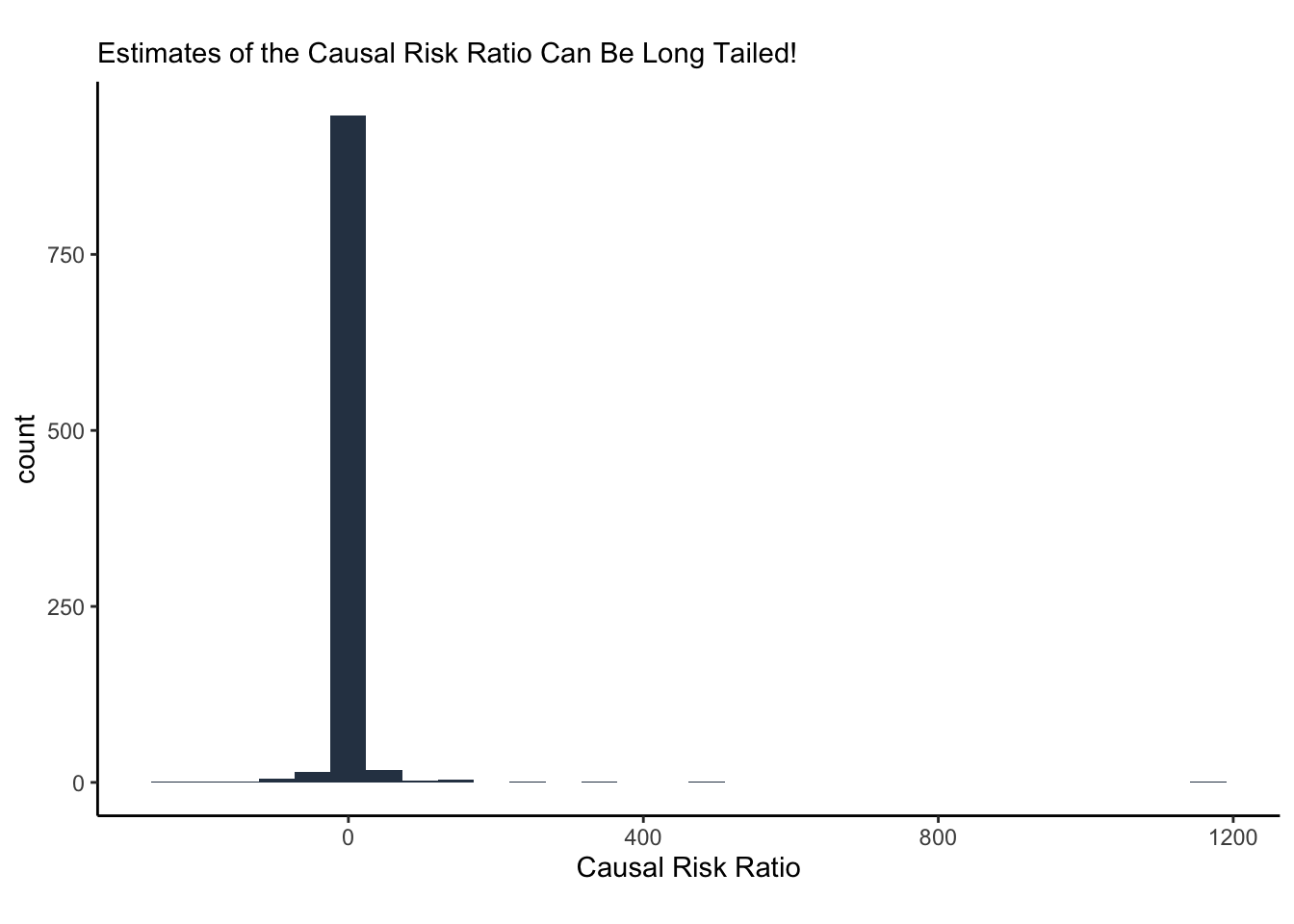
LMAO look at that tail! The long tail us due to the problems I’ve highlighted. In fact, we can highlight the “Oh shit zone” on a plot of the bootstraps (below in the figure below). The red line is where the tail behavior comes from; if you have a bootstrap replicate on that line, you should be saying “oh shit”.

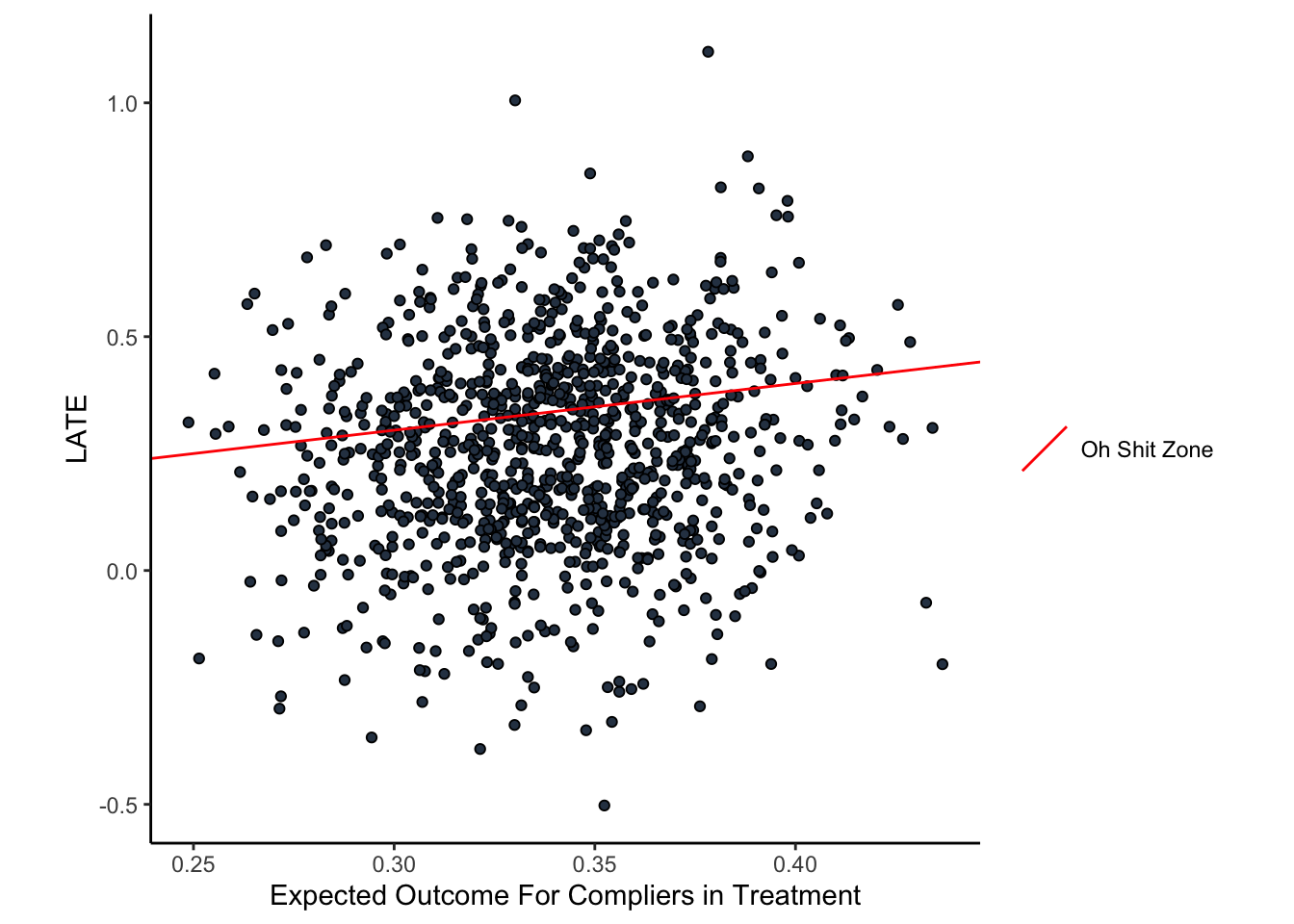
In fact, there are some estimates from the bootstrap which yield \(E[y^0\mid d^1]<0\) so… what was the point if this?

What Was The Point Of This Post

Ok, so estimating the causal risk ratio in a randomized experiment with one sided non-compliance is technically possible, but the math can get…weird. In particular, bootstrapping the standard errors (which is probably the most sensible way of estimating the standard errors unless you’re a glutton for delta method punishment) shows that we can get non-nonsensical bootstrapped estimates of the counterfacutal average outcome for compliers.

Honestly…I’m not sure where to go from here. Point estimates are possible but incomplete. Bootstrapping is a sanest way to get standard errors, but have no way of ensuring the estimates are bounded appropriately. All is not lost, its nice to know this sort of thing can happen. Maybe the most sensible thing to say here is “do not ask for causal risk ratios for these types of experiments” and that is worth its weight in gold.