I recently wrote a blog post for my employer in which I made some claims regarding Bayesian statistics.

Claim 1: Flat Priors in Heirarchal Models Can Lead to Pulling Apart and Implausible Estimates

On flat priors in hierarchical models, Gelman says

A noninformative uniform prior on the coefficients is equivalent to a hierarchical N(0,tau^2) model with tau set to a very large value. This is a very strong prior distribution pulling the estimates apart, and the resulting estimates of individual coefficients are implausible.

By “pulling the estimates apart” I assume Gelman means “not pooling/regularizing estimates” as opposed to literally pulling the estimates apart. As for the line about “implausibility” of individual coefficients, that requires some unpacking.

Gelman is known for picking out poor methodological papers and commenting on them. Consider “The prior can often only be understood in the context of the likelihood” in which Gelman and authors discuss a study which ostensibly demonstrated that “beautiful” people are more likely to have a daughter.

You’re free to read what Gelman and authors wrote, I won’t summarize it here, but in short the authors to which Gelman refers report an unusually high differential in the probability of giving birth to a girl if you are a “beautiful” person. Given what we know about the sex ratio of births and how they vary across the globe, this seems fairly extreme. Reading between the lines, I would go so far as to say Gelman would consider this estimate as “implausible”. Hence, I interpret “implausible” to mean “no different than Frequentist estimates”. That is not to say that all frequentist estimates are implausible, just that when certain estimates should be shrunk/regularized, a hierarchical model with a flat prior would fail to do so.

This is fairly easily demonstrated. I’m going to simulate 16 A/B tests. Each test is powered to detect a lift of 5%. However, each of the lifts from the 16 tests is drawn from a normal distribution with mean 1 and standard deviation 0.02. This means that, while not impossible to see a 5% lift, it is highly improbable and often our tests are underpowered for the true effect. This, as I understand it, is the prevailing attitude in A/B testing.

Each A/B test will be fed to a hierarchical model (shown below in Stan). I place a flat prior on the population mean and parameterize the prior on the population variance so that I can study how estimates change when the prior is less/more variable.


data{
  int n;
  vector[n] log_rr;
  vector[n] stderr;
  real beta;
}
parameters{
  real mu;
  real<lower=0> tau;
  vector[n] z;
}
transformed parameters {
  vector[n] theta = mu + tau * z;
}
model {
  // No mu in the model block means a uniform prior over the domain.
  tau ~ inv_gamma(3, beta);
  z ~ std_normal();
  log_rr ~ normal(theta, stderr);
}

Code

library(tidyverse)
library(cmdstanr)
library(tidybayes)

set.seed(0)

control_conversion <- 0.1
target_lift <- 1.05
target_conversion <- control_conversion * target_lift
design <- power.prop.test(p1 = control_conversion, p2 = target_conversion, power = 0.8)
n_per_group <- ceiling(design$n)
n_experiments <- 16

results <- replicate(n_experiments, {
  # In reality, we generate smaller effects than we wish we did
  actual_lift <- rnorm(1, 1, 0.02)
  actual_log_rr <- log(actual_lift)
  
  control <- rbinom(1, n_per_group, control_conversion)
  treatment <- rbinom(1, n_per_group, control_conversion * actual_lift)
  
  # Since the groups are the same size the two factors of log(n_per_group) cancel
  observed_log_rr <- log(treatment) - log(control)
  # A Standard result from the Delta method.
  sampling_var <- 1 / treatment + 1 / control - 2 / n_per_group
  stderr <- sqrt(sampling_var)
  
  c(observed_log_rr, stderr, actual_log_rr)
  
})

log_rr <- results[1, ]
stderr <- results[2, ]
actual_log_rr <- results[3, ]

# Keep track of the RMSE from our frequentist estimates.
# Hopefully, the Hierarchical model will do better than this.
observed_rmse <- sqrt(mean((log_rr - actual_log_rr) ^ 2))

model <- cmdstan_model('model.stan')

beta <- 10 ^ seq(-3, 4, 0.5)
sims <- map_dfr(beta, ~ {
  stan_data <- list(
    n = n_experiments,
    log_rr = log_rr,
    stderr = stderr,
    beta = .x
  )
  
  capture.output(
  fit <- model$sample(
    stan_data,
    parallel_chains = 10,
    adapt_delta = 0.99,
    chains = 10,
    refresh = 0, 
    seed=0
  )
  )
  
  
  estimated <- fit$summary('theta')$mean
  error <- actual_log_rr - estimated
  rmse <- sqrt(mean(error ^ 2))
  max_rhat <- max(posterior::summarise_draws(fit$draws('theta'), 'rhat')$rhat)
  divs <- sum(fit$diagnostic_summary()$num_divergent)
  
  tibble(rmse, beta = .x, max_rhat, divs)
  
})

stopifnot(all(sims$divs==0))
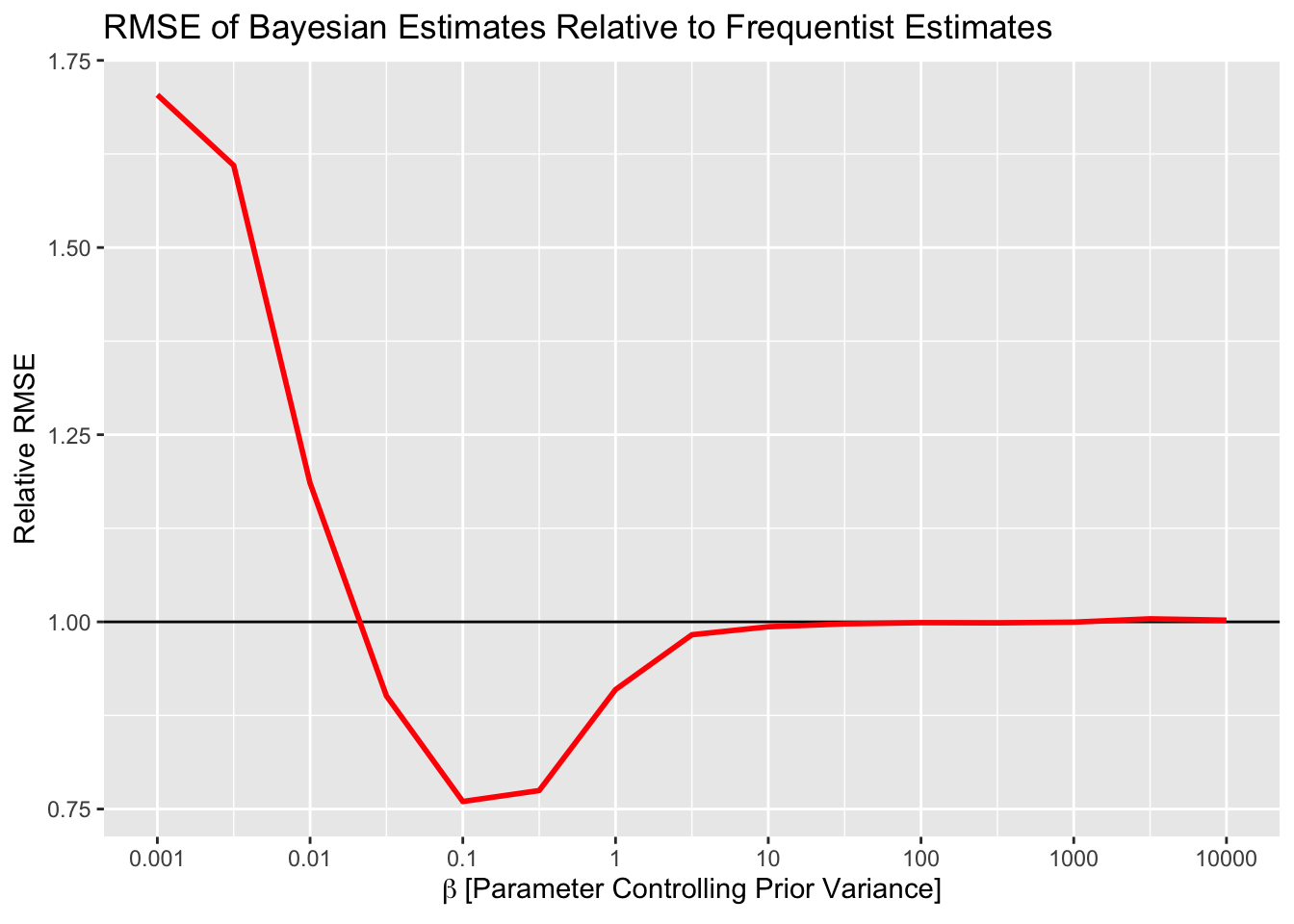
stopifnot(all(sims$max_rhat<1.01))

Below is a plot of the relative RMSE of the estimates from the Bayesian model. I’ve rescaled the y axis so that the black line (y=1) corresponds to the RMSE from the Frequentist estimates. As you can see, more informative priors do result in better RMSE – to a point. When the prior becomes too informative, then the RMSE increases. This is due to pooling all estimates to the grand mean. Conversely, when the prior on the variance is too large, no pooling happens and results are the same as Frequentist estimates (i.e. implausible if they are noisy a la Gelman).

So, let’s take stock. From this little simulation – which adheres the best I can to what I know about A/B testing, and is still imperfect – we have seen:

It is true that uninformative priors will give you equivalent estimates to Frequentist approaches (at least in terms of RMSE).
You probably don’t want to be similar to Frequentist results if you can help it, because you can do better (again in terms of RMSE) by applying a little prior information.
You don’t even need to be that accurate with your priors. Any reduction in RMSE is good, you don’t need to find the optimal prior to reduce the RMSE. In this case, anywhere between \(\beta = 0.05\) and \(\beta = 3\) is probably sufficient to reduce RMSE.
Setting a good prior (in this case) isn’t even that hard. Think about how variable individual experiments vary in results. You aren’t likely to see many experiments 1 lift unit away from the mean. You know, intuitively, that lift estimates are probably somewhere between -10% and 10% on a good day. Even if you were REALLY uncertain and said -50% to 50% for any given experiment, that is still a standard deviation of ~25% and hence well within the range of reducing RMSE (again, in this example. I can’t say if this applies generally).

Listen, Bayesian or Frequentist, I don’t care. However, it is absolutely clear that, when you pay careful attention to the nuance, the difference between Bayes and Frequentism is a big deal despite what some will say.