Important
In accordance with my AI policy, I have written this blog post myself. However, all code is written Claude and a lot of the mathematics is done in conjunction with Gemini.
Introduction
I’ve been thinking about the hierarchical normal-normal model a lot recently. We’re planning to build some sort of empirical Bayes estimation service for a variety of reasons (I won’t expound on the virtues of shrunken estimates here). The question is how best to do this given the imperfectness of real data.
One little hurdle I’ve hit is what to do with experiments which have multiple variants. Because effect measures from the same experiment share a control group, they are correlated, and that introduces a little bit of complexity into the model. To see why, let’s consider three effect measures which come from 3 separate and independent experiments. Assuming we know the standard errors for those effect measures perfectly, then the likelihood for the model can be thought of as multivariate normal
\[\begin{bmatrix} \delta_1 \\ \delta_2 \\ \delta_3 \end{bmatrix} \sim \operatorname{MVNormal} \left( \begin{bmatrix} \theta_1 \\ \theta_2 \\ \theta_3 \end{bmatrix}, \begin{bmatrix} s^2_1 & 0 & 0 \\ 0 & s^2_2 & 0 \\ 0 & 0 & s^2_3 \end{bmatrix} \right) \>.\]
Now, suppose that \(\delta_1\) and \(\delta_2\) come from the same experiment, hence they share a control group. It is straight forward to show that if \(\delta\) is a difference in means, then the covariance is
\[ \operatorname{Cov}(\delta_1, \delta_2) = s^2_c \>.\]
Here, \(s^2_c\) is the sampling variance for the average outcome in the control group for that experiment. This means that the likelihood, as a multivariate Gaussian, would be
\[\begin{bmatrix} \delta_1 \\ \delta_2 \\ \delta_3 \end{bmatrix} \sim \operatorname{MVNormal} \left( \begin{bmatrix} \theta_1 \\ \theta_2 \\ \theta_3 \end{bmatrix}, \begin{bmatrix} s^2_1 & s^2_c & 0 \\ s^2_c & s^2_2 & 0 \\ 0 & 0 & s^2_3 \end{bmatrix} \right) \>.\]
Clearly, these two models have different likelihoods. My pragmatic solution is to sample a single effect measure from each experiment. This ensures the covariance in the likelihood is diagonal. Do I have to do this? What do I have to pay when I assume all effect measures are independent, even when they are correlated? When does the correlation become something I have to model?
I’ve worked with Gemini (which I find understands my style a little better than ChatGPT when it comes to math) to poke and prod at this question a little. Together, we’ve determined a few criteria under which the naive approach of modelling all effect measures as independent would lead to the wrong outcome. Below, I demonstrate some fairly extreme and unrealistic examples, just for the sake of exposition.
Setup
Let’s set up the problem more concretely. Say I have \(K\) experiments, where experiment \(k\) has \(n_k\) effect measures (comparisons against treatment, which we will assume are differences in means for now). Let \(\delta_{k,i}\) denote the effect measure for variant \(i\) against control in experiment \(k\), for \(k = 1, \ldots, K\) and \(i = 1, \ldots, n_k\). Stacking all \(N = \sum_k n_k\) effect measures into a single vector \(\delta\), the hierarchical normal-normal model is
\[\delta \sim \operatorname{MVNormal}(\theta, \Sigma)\] \[\theta \sim \operatorname{MVNormal}(\mu, \tau^2 I)\]
where \(\Sigma\) is a block-diagonal matrix. For experiments with a single variant, the corresponding block is just the scalar sampling variance \(s^2_{k,1}\). For experiments with multiple variants, the block for experiment \(k\) has diagonal entries \(s^2_{k,i}\) and off-diagonal entries \(s^2_{c,k}\) (the sampling variance of the control mean in experiment \(k\)). For example, if \(K = 3\) with \(n_1 = 3\), \(n_2 = 2\), and \(n_3 = 1\), then
\[\Sigma = \begin{bmatrix} s^2_{1,1} & s^2_{c,1} & s^2_{c,1} & 0 & 0 & 0 \\ s^2_{c,1} & s^2_{1,2} & s^2_{c,1} & 0 & 0 & 0 \\ s^2_{c,1} & s^2_{c,1} & s^2_{1,3} & 0 & 0 & 0 \\ 0 & 0 & 0 & s^2_{2,1} & s^2_{c,2} & 0 \\ 0 & 0 & 0 & s^2_{c,2} & s^2_{2,2} & 0 \\ 0 & 0 & 0 & 0 & 0 & s^2_{3,1} \end{bmatrix}\]
Writing the marginal likelihood by integrating out \(\theta\), we get
\[\delta \sim \operatorname{MVNormal}(\mu \cdot \mathbf{1}, \Sigma + \tau^2 I)\]
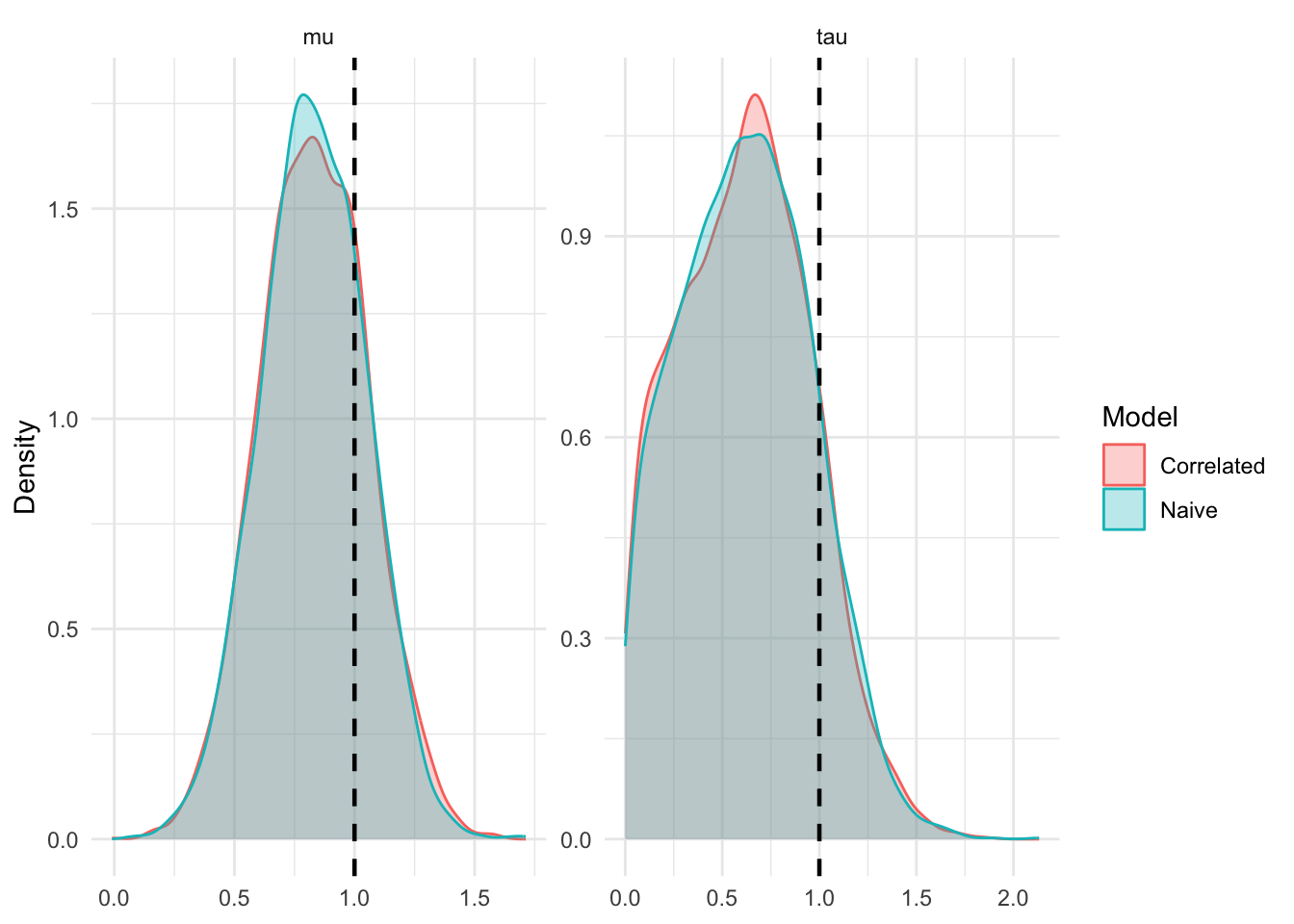
We can sample from this model using stan. When the \(\delta\) truly are independent, MCMC works fine. I simulate \(K=50\) experiments, each with \(n_k=1 k = 1, \ldots, 50\) effect estimates.
Now that we have set up our problem, let’s discuss when and how treating the elements of \(\delta\) as independent can fail.
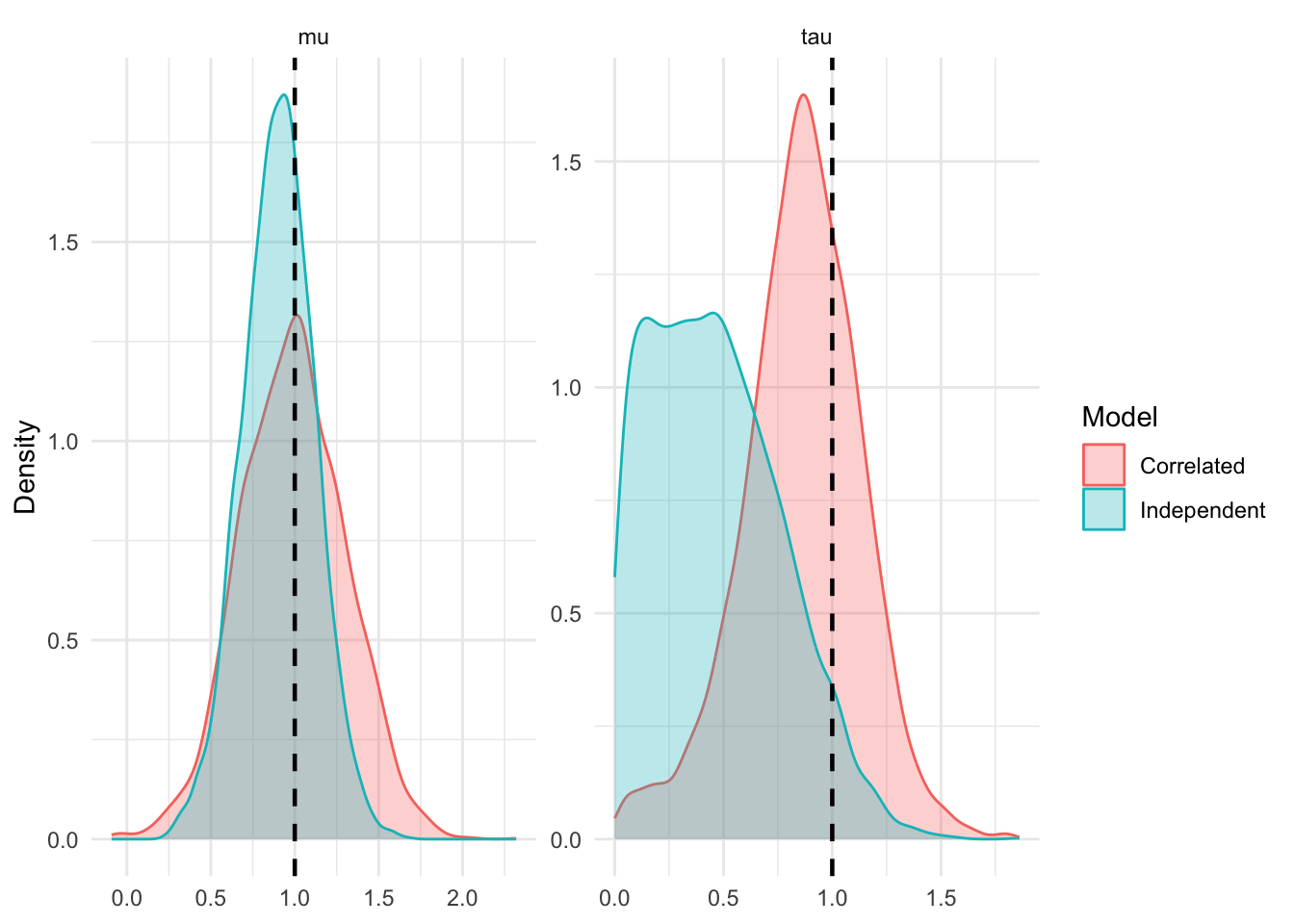
1. You’ve Got A Single Experiment With A Lot of Variants
Let’s focus on the block of the covariance matrix associated with experiment \(k\). Let’s assume the sampling variance for the treatment arms in this experiment are roughly equal, such that \(s^2_{k,i} = s^2_t + s^2_{c,k}\) for all \(i = 1, \ldots, n_k\).
The \(n_k \times n_k\) marginal covariance block for this experiment, \(V_k\), incorporates the treatment sampling variance, control sampling variance, and between-arm heterogeneity \(\tau^2\): \[V_k = (s^2_t + \tau^2) I_{n_k} + s^2_{c,k} \mathbf{1}_{n_k} \mathbf{1}_{n_k}^T\]
For economy of thought, let \(v = s^2_t + \tau^2\). We can invert this matrix using the Sherman-Morrison formula: \[V_k^{-1} = \frac{1}{v} I_{n_k} - \frac{s^2_{c,k}}{v(v + n_k s^2_{c,k})} \mathbf{1}_{n_k} \mathbf{1}_{n_k}^T\]
The total precision this experiment provides for estimating \(\mu\) is the sum of all elements in the inverse covariance matrix, \(\mathbf{1}_{n_k}^T V_k^{-1} \mathbf{1}_{n_k}\). We can derive this exactly:
\[ \begin{align*} \mathcal{I}_{corr} &= \mathbf{1}_{n_k}^T \left( \frac{1}{v} I_{n_k} - \frac{s^2_{c,k}}{v(v + n_k s^2_{c,k})} \mathbf{1}_{n_k} \mathbf{1}_{n_k}^T \right) \mathbf{1}_{n_k} \\ &= \frac{n_k}{v} - \frac{n_k^2 s^2_{c,k}}{v(v + n_k s^2_{c,k})} \\ &= \frac{n_k (v + n_k s^2_{c,k}) - n_k^2 s^2_{c,k}}{v(v + n_k s^2_{c,k})} \\ &= \frac{n_k v}{v(v + n_k s^2_{c,k})} \\ &= \frac{n_k}{v + n_k s^2_{c,k}} \end{align*} \]
Note that this quantity is bounded above \[\lim_{n_k \to \infty} \mathcal{I}_{corr} = \lim_{n_k \to \infty} \frac{n_k}{v + n_k s^2_{c,k}} = \frac{1}{s^2_{c,k}}\]
This means that no matter how many treatment arms you add to experiment \(k\), the information it contributes to \(\mu\) is strictly upper-bounded by the precision of the shared control group.
If we naively assume independence, the off-diagonal terms \(s^2_{c,k}\) are zeroed out in \(\Sigma\). The total information becomes the sum of \(n_k\) independent precisions: \[\mathcal{I}_{indep} = \frac{n_k}{v + s^2_{c,k}}\] As \(n_k \to \infty\), the naive model’s information \(\mathcal{I}_{indep} \to \infty\). By treating elements of \(\delta\) as independent, the model becomes overconfident, allowing a single experiment to entirely dominate the hyper-parameter estimates.
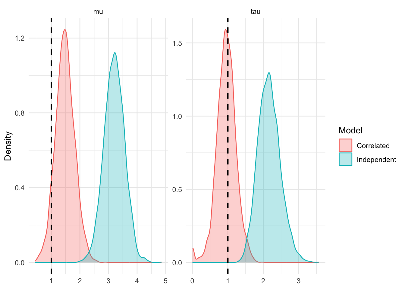
2. The Control Is Estimated With A Lot of Error
Suppose the true mean of the control group in experiment \(k\) is \(\mu_c\), but due to sampling variance, the observed mean is drawn with a massive negative error. Consequently, all \(n_k\) observed effect measures \(\delta_{k,i}\) will be artificially inflated.
In the marginal log-likelihood, the penalty term for experiment \(k\) is proportional to: \[- \frac{1}{2} (\delta_k - \mu \mathbf{1}_{n_k})^T V_k^{-1} (\delta_k - \mu \mathbf{1}_{n_k})\]
Looking back at our derivation of \(V_k^{-1}\), the off-diagonal elements are exactly: \[- \frac{s^2_{c,k}}{v(v + n_k s^2_{c,k})}\]
These strictly negative off-diagonal terms discount the shared anomaly. When computing the quadratic form, the cross-terms subtract value away from the likelihood if multiple \(\delta_{k,i}\) deviate from \(\mu\) in the same direction. A simultaneous shift of all \(n_k\) arms is highly unlikely unless it was driven by the shared variance component \(s^2_{c,k}\).
If we assume an independent, diagonal \(\Sigma\), these negative correcting terms disappear. The model receives \(n_k\) independent signals that the treatment effect is larger than it was in reality, leading to potential bias in \(\mu\) and \(\tau\).
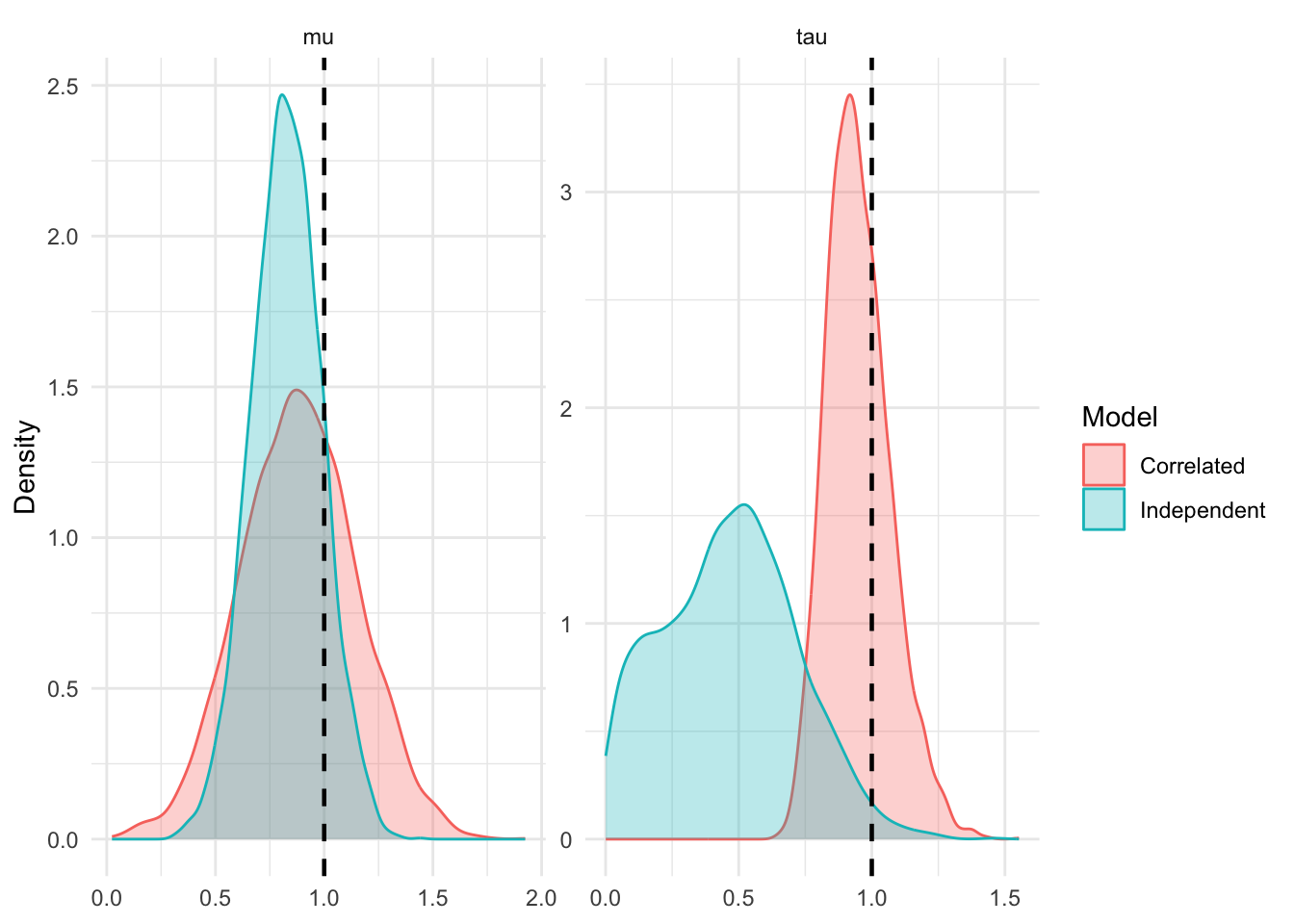
3. Your Propensity Score Highly Favors the Variant Over The Treatment
The degree to which we have to model the correlation depends on the ratio of the control sampling variance to the treatment sampling variance.
For any two variants \(i\) and \(j\) in experiment \(k\), the correlation of their effect measures in the likelihood is: \[\rho_{i,j} = \frac{s^2_{c,k}}{\sqrt{(s^2_{t,k,i} + s^2_{c,k})(s^2_{t,k,j} + s^2_{c,k})}}\]
If \(s^2_{t,k,i} \approx s^2_{t,k,j}\), this simplifies to: \[\rho \approx \frac{s^2_{c,k}}{s^2_t + s^2_{c,k}}\]
This gives us an idea of when the approximation is safe. If the control group has the majority of traffic then \(s^2_{c,k}\) will be tiny compared to the treatment variance \(s^2_t\). The correlation approaches zero, \(\Sigma\) becomes essentially diagonal, and sampling a single effect measure throws away valuable, nearly-independent information. If the treatment has the majority of traffic, \(s^2_{c,k}\) dominates \(s^2_t\). The correlation approaches 1. The effect measures are almost perfectly co-linear, and treating them as independent should severly bias estimates.
Conclusion
This has been a good exercise in understanding the limitations of a simple model. I still think I’m going to sample a single variant for each experiment, mostly because it seems like a defensible way to keep things simple and avoid checking conditions like this. That being said, I don’t think many experimentation programs would meet any of these criteria. For one thing, experiments usually have 2-5 variants (from the ones I have seen), and so the first scenario is less likely. Even if we did get a single experiment with dozens of variants, seems like the limiting factor is the precision in the control – which can be very large in the experiments we see. Additionally, if there was any reason to believe the control was measured with a lot of error, then perhaps the experiment should be excluded as opposed to included in the model. Lastly, a lot of experiments are either going to do a 50/50 split or bias traffic towards control as opposed to treatment (perhaps with the exclusion of holdouts? I’m not completely sure).
All this to say, even if I didn’t sample a single variant per experiment, I’m not sure the difference would be material.