Important
This blog post is inspired, almost entirely, by Tyler Buffington’s excellent statistics reading group presentation today at Datadog on the value of information in A/B testing. The ideas presented here are mainly his, I’ve just gone ahead and done a little more math. I’ve also relied a lot on AI to help me get through some of the math. I can’t remember all the tricks there are for manipulating expectations and bivariate normals, and so AI as been helpful here. In accordance with my AI page, all writing is in my own voice and I have used AI extensively to write simulation code.
Introduction
In this post, I discuss decision criteria for Bayesian A/B testing and a way to think about experiment run times for Bayesian A/B tests. I’ll also present some analytic results that can help us avoid doing simulations in practice at the cost of some mild assumptions.
First, I’ll discuss a little background on some straightforward ways to analyze A/B tests as a Bayesian and discuss a few options for ship/no-ship decision rules for A/B tests. Then, I’ll introduce a way to think about expected impact as a Bayesian, and finally share some analytic results.
Bayesian Approaches to A/B Testing
Most A/B tests target the lift in a metric, defined as
\[ \lambda = \dfrac{E[Y(1)]}{E[Y(0)]} - 1 \>. \]
We can obtain an estimate of the lift, \(\hat \lambda\), via the plug in principle and the associated standard error, \(s_\lambda\) via the delta method. Assuming \(\hat \lambda\) is drawn from a normal distribution (I’ve talked about this before here), and that \(s_\lambda\) is known exactly, we can use a conjugate normal-normal model to obtain the posterior distribution. Assuming the prior mean and variance is \(\mu\) and \(\tau^2\) respectively, the posterior variance and mean, \(V\) and \(M\), are
\[ V^{-1} = \dfrac{1}{s^2_\lambda} + \dfrac{1}{\tau^2} \>, \] \[ M = V \times \left(\dfrac{\hat \lambda}{s^2_\lambda} + \dfrac{\mu}{\tau^2}\right) \>. \]
Whereas a Frequentist would make their ship/no-ship decision based on statistical significance, a Bayesian has a few options. Assuming increases to the metric are favorable, many of the decision rules are based on inequalities of the posterior mean. Here are just three I have seen in the wild:
- Ship if \(c \lt \Pr(\lambda \gt 0 \mid \hat \lambda)\), which is equivalent to \(\sqrt{V} \Phi^{-1}(c) \lt M\), where \(\Phi\) is the standard normal CDF. This is sometimes called “Probability to beat control”.
- Ship if \(z_{1-\alpha/2}\sqrt{V} \lt M\). This is like a Bayesian p-value being less than \(\alpha\).
- Ship if \(0 \lt M\). Ship whenever the posterior mean is positive.
Now, these are just a few ways to make decisions (they are certainly not exhaustive). Prior to Tyler’s talk, I didn’t really have a great way to answer how long an A/B test should take (save some ramblings about EVSI here) were you to use a Bayesian analysis method. However, with these details, I think I can now give an answer.
How Long To Run an A/B Test as a Bayesian
The question of how long to run an A/B test is really a question of sample size. Assuming you accrue some number subjects per week, you can do some back of the napkin math to say how long the test should run to sufficiently power the experiment given an MDE and some information on the metric. Often, we flip the script and present MDEs as a function of time (e.g. if you want a 3% MDE, run this experiment for 2 weeks. Want a smaller MDE? Run it longer). Run length is now a knob one can tune.
This is do-able as a Frequentist because we have a very clear relationship between power, MDE, and sample size (which is a function of time). Although there are Bayesian conceptions of power (e.g. conditional power, unconditional power, etc etc), the formulae for these don’t so straightforwardly relate time and desired effect sizes. This is further complicated by the prior – if your prior says a 5% lift is not probable, you probably shouldn’t design experiments to detect 5% lifts.
Rather than seek a formula right now, we can first draw random numbers to see what happens under different scenarios. Consider the following algorithm:
- Draw a true lift from your prior, \(\lambda\).
- Draw a control group mean from the implied sampling distribution (you need the control mean and standard error to do this, but you should know this if you were going to do a power calculation anyway).
- Draw a treatment group mean from the implied sampling distribution.
- Compute \(\hat \lambda\) and \(s_\lambda\)
- Compute \(M\) and \(V\).
- Apply your decision rule. If you reach ship criteria, then return the true lift, else return 0.
- Repeat a few thousand times.
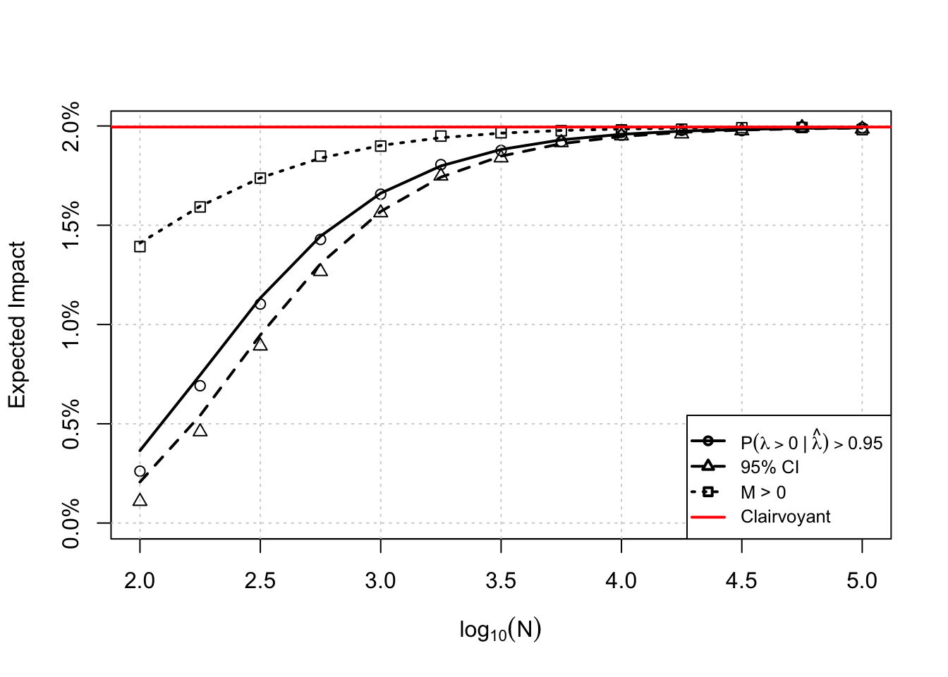
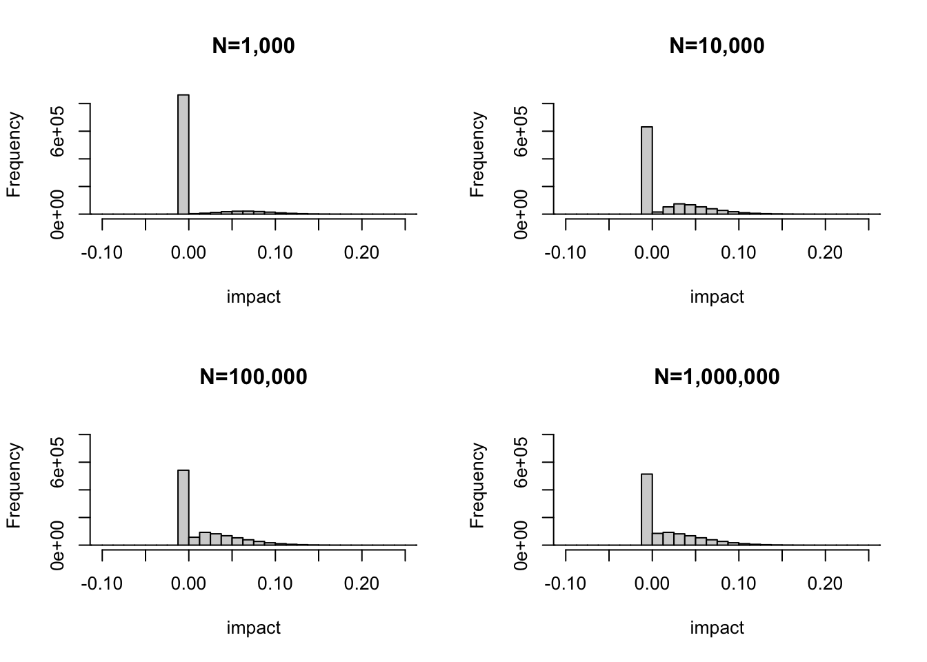
Here, time affects the sampling distributions of treatment and control. The longer the experiment runs, the more samples we accrue, the larger the precision in the group means will be. This procedure is shown for 4 scenarios below. The histograms show the distribution of true impacts to the product under the decision rule. The large spike at 0 indicates those A/B tests which resulted in no ship decisions, and the remainder are the impacts from shipping.
Note a few things. First, while difficult to see, there are some cases (especially in small sample sizes) where we ship harm to the product! This makes sense, when we have noisy measurements sometimes we can make type \(S\) errors. As the sample size increases, the probability we make these errors decreases as does the proportion of no-ship decisions (the height of the spike decreases). Second, the mean of this distribution is the “average impact to the product”. This mean changes slightly due to my first point, and eventually the distribution of these impacts stabilizes to some limiting distribution (Tyler referred to this as the Clairvoyant distribution, essentially the distribution of impacts were you to know the true lift perfectly). Hence, there is some upper bound to the mean.
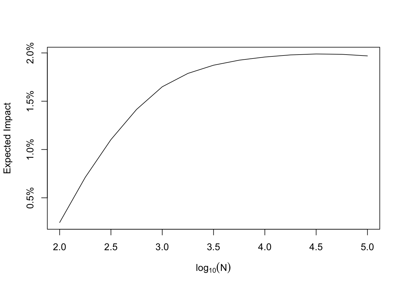
Below is a plot of the mean of this distribution as a function of sample size, and you can see this limiting behavior quite clearly. The proposal is to base your run time on the expectation of the Clairvoyant distribution. From the plot, running A/B tests too short means the impact is going to be very small on average, but running longer means that (under the prior) you will impact the product more. There comes a point where running the test longer is not helpful because you encounter diminishing returns. This is a nice way to think about run time in my opinion! You know what your average impact would be were you to have perfect information, and you can collect enough samples so that you are sufficiently close to this without wasting time obtaining additional samples. I think that is pretty elegant!
Note that I’ve just shown simulations for probability to beat, but the simulation approach is sufficiently flexible to accommodate any decision rule (expected loss, Bayesian p values, or whatever you can cook up). If you’re an analyst, you can do this fairly readily on your computer. What if you wanted to make this a product many people can use, and use with reproducible results? Simulating is fine in my opinion, generating random numbers and counting should be pretty cheap, but it would be cool to have a formula for the expected value of this distribution as a function of the total sample size.
An Analytic Solution
Simulation is great to get some intuition for what is happening, but we can actually recover these curves analytically with a little effort. First, note that all three of the decision rules are of the form
\[ \sqrt{V}\Phi^{-1}(p) \lt M \>. \]
For the three decision rules I’ve listed above, \(p = c\), \(p=1-\alpha/2\), and \(p=0.5\).
With some algebra, we can express this inequality in terms of the observed lift \(\hat \lambda\), which would be
\[S(N) = s_\lambda^2 \left[ \Phi^{-1}(p) \sqrt{\frac{1}{\tau^2} + \frac{1}{s_\lambda^2}} - \frac{\mu}{\tau^2} \right] \lt \hat \lambda\]
Note that \(s_\lambda^2\) implicitly relies on \(N\) via the standard errors for treatment and control. Now, technically, \(s^2_\lambda\) relies on the estimated lift \(\hat \lambda\), but in practice the lifts are small (we don’t routinely detect enormous hurt/help to the product). This seems to be the prevailing opinion in the A/B testing literature and community, and so I’m going to hand wave this detail away.
We want to calculate the expected true impact \(\lambda\) given that we observe a signal \(\hat \lambda\) strong enough to ship:
\[E[\text{impact} \mid N] = E[\lambda \cdot \mathbf{1}\{\hat \lambda > S(N)\}]\]
Under our model, the joint distribution of the true effect and the observed effect is bivariate normal:
\[\begin{pmatrix} \lambda \\ \hat \lambda \end{pmatrix} \sim \mathcal{N} \left( \begin{pmatrix} \mu \\ \mu \end{pmatrix}, \begin{pmatrix} \tau^2 & \tau^2 \\ \tau^2 & \tau^2 + s_\lambda^2 \end{pmatrix} \right)\]
Using the properties of the multivariate normal distribution, the expected value of \(\lambda\) over the truncation \(\hat \lambda > S(N)\) is
\[E[\lambda \cdot \mathbf{1}(\hat \lambda > S(N))] = \mu \Phi(a) + \frac{\tau^2}{\sqrt{\tau^2 + s_\lambda^2}} \phi(a) \>.\]
Here, \(a\) is
\[a = \frac{\mu - S(N)}{\sqrt{\tau^2 + s_\lambda^2}} \>.\]
Substituting \(S(N)\) back into our expression for \(a\) gives a fully analytic expression for expected impact as a function of sample size
\[E[\text{impact} \mid N] = \mu \Phi\left( \frac{\mu - S(N)}{\sqrt{\tau^2 + s_\lambda^2}} \right) + \frac{\tau^2}{\sqrt{\tau^2 + s_\lambda^2}} \phi\left( \frac{\mu - S(N)}{\sqrt{\tau^2 + s_\lambda^2}} \right)\]
As a corollary, we can obtain the Clairvoyant impact (the impact with perfect information). As \(N \to \infty\), the sampling variance \(s_\lambda^2 \to 0\). In this limit, \(S(N) \to 0\) and so the expression collapses to the mean of a folded or truncated normal distribution
\[E[\text{Clairvoyant impact}] = \mu \Phi\left( \frac{\mu}{\tau} \right) + \tau \phi\left( \frac{\mu}{\tau} \right)\]