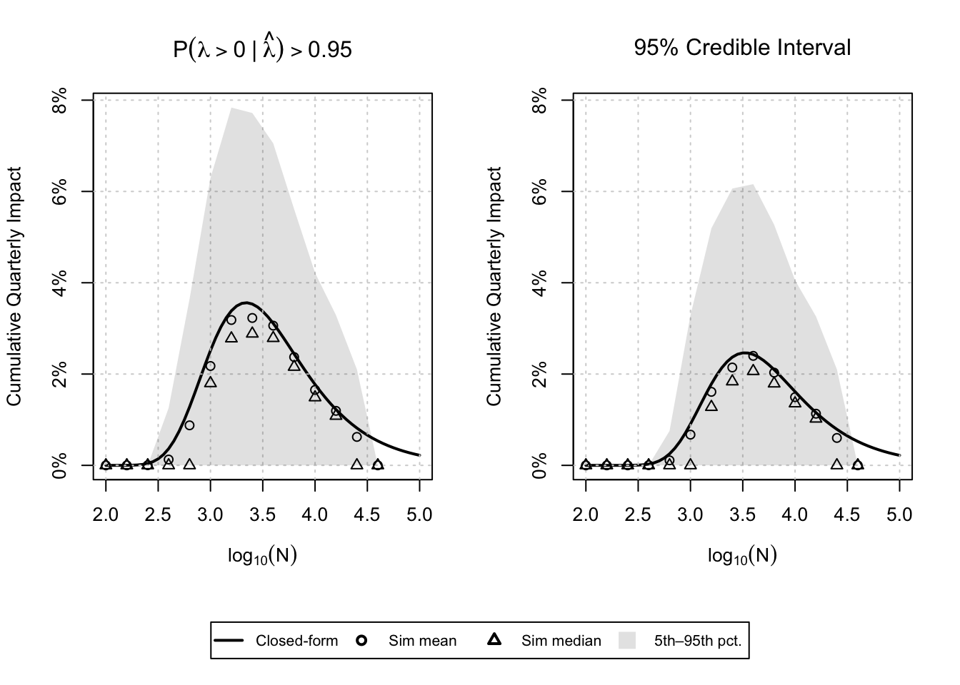
This post is a spiritual successor to an early post on this blog and a fast follow here from this post about A/B test run times for Bayesians. From that post, we are able to obtain an analytic approximation to the expected impact from a single experiment using a Bayesian analysis and a given decision rule. Below is a plot like the one found in my other post, but this time perhaps with a more realistic prior.
These curves tell me what my expected impact is going to be at given sample sizes, but not what sample size I should choose. Obviously, I want to impact the product as much as possible, but I don’t want to spend months and months on a single experiment.
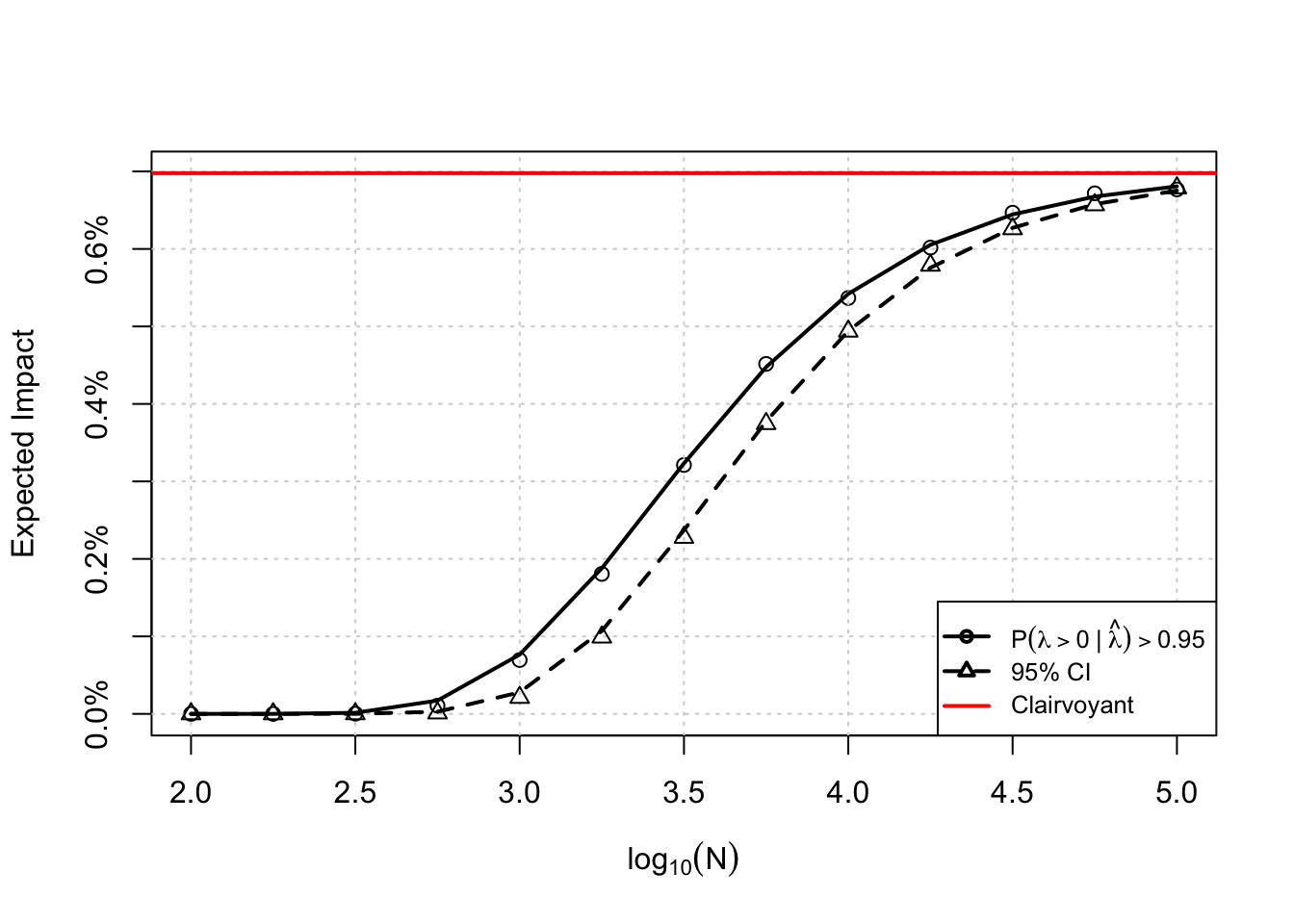
Let’s assume I can accrue \(N\) total subjects per week. I can either choose to run more experiments at a lower expected impact, or run fewer experiments with higher impact. Remember, not every experiment is going to be a “ship” decision, this expected impact is over all experiments. There should be some sweet spot where I am running sufficiently many experiments with sufficiently high impact. Intuitively, this should be the sample size we choose for our A/B tests. For the curves above, the plot I describe looks something like the one shown below.
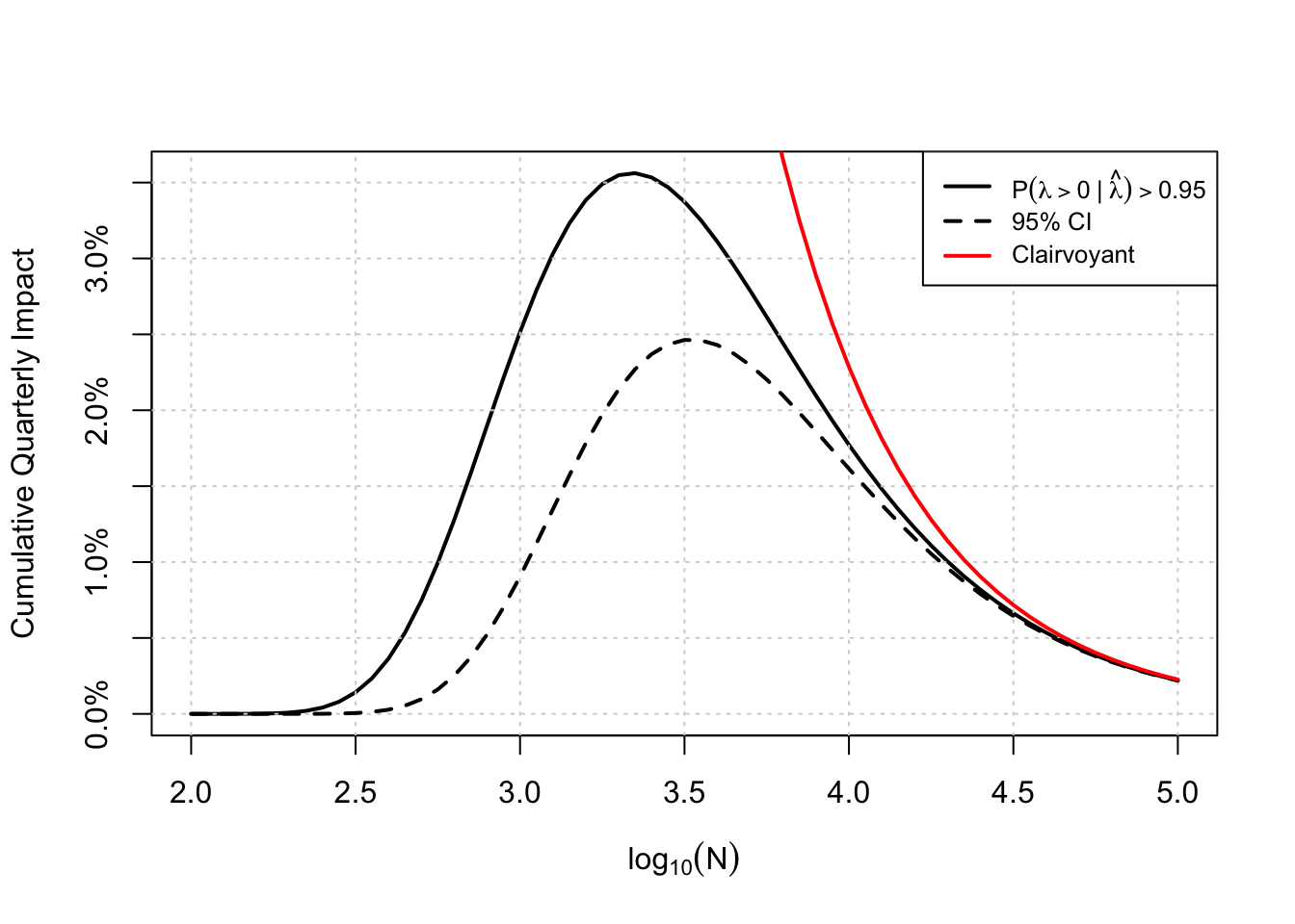
From this plot, we learn a few things: First, the decision rule to ship only if the credible interval excludes 0 is dominated by the probability to beat decision rule in both quarterly expected impact (at least for the parameters I’ve used here), and we can achieve higher impact with fewer samples per experiment (roughly 780 fewer assuming the optima are at \(\log_{10}(N)=3.25\) and 3.5 respectively). The one thing this plot is missing is some sort of uncertainty for these curves – remember, these are expectations and the true cumulative impact is going to vary about these points, perhaps drastically so! I think that is a better job for simulation.