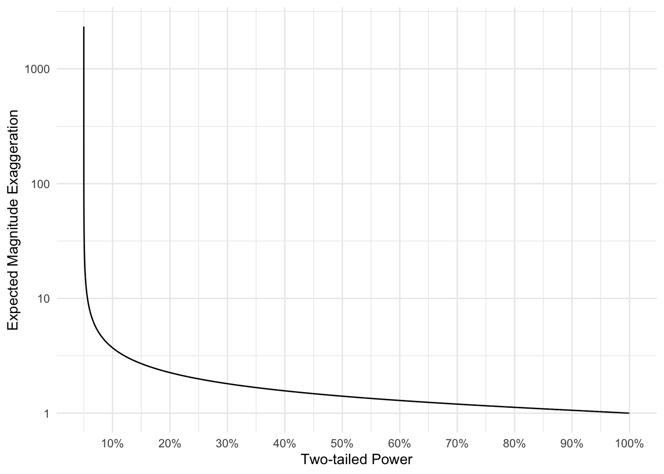
I want to start this post at the end: statistically significant results from low powered experiments are, almost certainly, an exaggeration to the truth.
Below, I show the expected amount by which a statistically significant result will exaggerate the truth as a function of the statistical power (note the log scale). This means at 80% power, we should expect statistically significant results to exaggerate the truth by a factor of roughly 13% (an often quoted fact by Ron Khohavi if I understand correctly). The remainder of this post will derive the formula for this curve and discussing implications.
This is not news. Lately, I’ve been trumpeting solutions to the Winner’s Curse, and I’ve posted about this exact topic here and here. So why report old news?
I recently gave a talk to some product analytics engineers about the sample size calculator we built for the experimentation product. My message was not exactly subtle: looking at two time series and claiming one group’s metric is better than another is a bad way to make decisions, and is especially bad when those decisions are made from small samples. Even if these decisions used statistical tests a la AB testing, they would very likely be under powered for the true effect (and this is not to say anything about peeking, always valid intervals, and the trade off of statistical power required therein).
I don’t think I really drove the point home for just how much the effect can be exaggerated.
I’ve included the derivation for the curve below.
Click here to see the derivation
Let \(\theta\) be the true treatment effect and suppose
\[ \hat{\theta} \sim N(\theta,s^2), \]
where \(s\) is treated as known. If positive effects are favorable and an estimate is detected when \(|\hat{\theta}|>cs\), define the expected exaggeration factor as
\[ R(\theta,s) = \frac{ E\left[|\hat\theta|\mid |\hat\theta|>cs\right] }{ |\theta| }, \qquad c=z_{1-\alpha/2}. \]
Here, for \(\theta>0\), \(\lambda = \theta / s\) is the signal to noise ratio. The stattistical power to exceed the detection threshold is
\[ p_+(\lambda) = P(\hat\theta>cs) = 1-\Phi(c-\lambda) \]
and
\[ p_-(\lambda) = P(\hat\theta<-cs) = \Phi(-c-\lambda). \]
Therefore,
\[ \pi(\lambda) = p_+(\lambda)+p_-(\lambda). \]
We can re-write this using the expectation of a truncated normal (see here) as
\[ E\left[\hat\theta\,1(\hat\theta>cs)\right] = \theta p_+(\lambda)+s\varphi(c-\lambda) \]
and
\[ E\left[-\hat\theta\,1(\hat\theta<-cs)\right] = -\theta p_-(\lambda)+s\varphi(c+\lambda). \]
Combining the tails gives
\[ R(\lambda) = \frac{ \lambda\left[p_+(\lambda)-p_-(\lambda)\right] +\varphi(c-\lambda) +\varphi(c+\lambda) }{ \lambda\left[p_+(\lambda)+p_-(\lambda)\right] }. \]